

When you want to apply formatting in Excel based on certain criteria, it’s called Conditional Formatting. This list of in-depth tutorials will help you find the answers you need so that you can learn and apply this useful function.
If you can’t find what you’re looking for or need answers fast, Excelchat is standing by to help 24/7.
How to Combine Conditional Formatting with an IF Statement
This tutorial shows you how to get conditional formatting in Excel using the IF statement in a custom formula. The condition syntax is the IF/THEN/ELSE formula to get your desired result. Not only do you get an example with images but also a video walkthrough of the process.
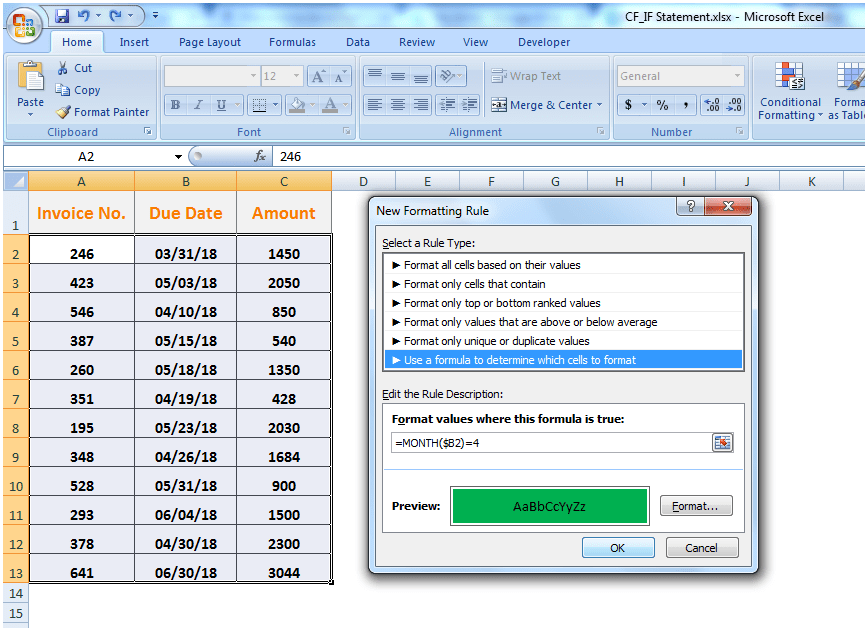
Learn how to use Conditional Formatting with an IF statement.
How to Use Conditional Formatting to Change Cell Background Color Based on Cell Value
Maybe you know how to change the color of a cell, but want to have the cells in your spreadsheet color-coded based on specific criteria. This article shows how to apply conditional formatting to change the background color of your cell based on a predetermined value.
Learn How to Copy and Paste Conditional Formatting to Another Cell
If you want to use the same conditional formatting in several places, this piece shows you how to copy and paste conditional formatting from one cell to another. There are several ways to accomplish this, and the tutorial illustrates them.
How to Apply Conditional Formatting to Blank Cells
Assuming you have blank cells or cells that don’t contain any values in Excel, you can also apply conditional formatting in these cases. This article not only shows you how to do this with step-by-step instructions and illustrations but also a video tutorial.
How to Use Conditional Formatting to Highlight Cells Less Than or Greater Than Some Value
Do you want to highlight cells based on certain criteria, such as something that is less than or greater than a specific value? This tutorial explains how to use conditional formatting to accomplish this, including images and a detailed video tutorial.
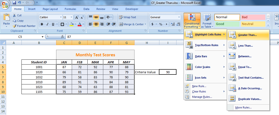
Learn how to apply conditional formatting to highlight cells less than or greater than a value.
Learn How to Apply Conditional Formatting Based on the Value of Another Cell
This tutorial shows you how you can use the value of another cell to apply conditional formatting. For example, you can highlight all cells a certain color if they fall below the yearly average. There are detailed instructions and illustrations to follow as a guide.
Highlight Dates in the Next N Days
Assuming you have a spreadsheet that is full of dates, you might need to find the ones that are coming up soon. You can learn how to highlight the dates in the next N days with this tutorial. It shows you how to set up the data and apply conditional formatting using the TODAY function.
Learn How to Use SUMIFS in Google Sheets
This is a tutorial that shows the reader how to use the SUMIFS function in Google Sheets. After going through this lesson, you’ll be able to sum a range of values and apply criteria to either exclude or include different values. There are examples and illustrations included.
How to Highlight a Row Using Conditional Formatting
If you have a spreadsheet filled with data and want to highlight a row based on certain criteria, this tutorial will show you how to do this by applying conditional formatting. By using examples and illustrations, it shows you how to create a condition that will result in your specified row being highlighted.
Learn How to Fill a Cell with Color Based on a Condition
This tutorial shows the reader how to fill a cell with a background color based on a condition or criteria. Using conditional formatting, you can create the criteria that you wish to match and the cell color. There are examples and illustrations for reference.

Find out how to fill a cell with a background color based on a condition.
Find Duplicate Values in Two Columns
This explanatory piece shows the reader how to find duplicate values in two columns in Excel. Specifically, it shows how to do this using the COUNTIF and AND functions, creating a separate list that identifies instances of duplicates.
Change Cell Color of Top 10 Values in a Column
If you need to create ranking lists in Excel and want to identify them visually, you can use conditional formatting. This tutorial shows how to change the cell color in a column by finding the top 10 values and highlighting them by the color of your choosing. It includes examples and illustrations.
How to Copy the Conditional Format to Another Cell
This is another tutorial that shows how you can use conditional formatting across various cells without having to re-create it each time. The step-by-step guide directs the reader on how to copy a conditional format for formulas, colors, and other formats from one cell to another using different methods.
How to Use the SUMIFS Function in Excel
This explanatory piece shows the syntax of the SUMIFS function in Excel, breaks down its different arguments and then provides a tutorial on its use. You will learn where you can and can’t use this function as well as how to use SUMIFS with comparison operators, using SUMIFS with cell references, with blanks, and wildcards.
How to Highlight Every Other Row in Excel
If you have a large spreadsheet or a lot of numbers, it might be easier to read if you highlight every other row in Excel. This requires the use of conditional formatting, and this tutorial shows you how to accomplish this in several ways.
Find out how to fill a cell with a background color based on a condition.
How to Normalize Text in Excel
If you want the text in your Excel spreadsheet to be consistent, you can “normalize” it in several different ways. This tutorial shows the reader how to normalize text in Excel with several examples and illustrations.
A Guide to Using Conditional Data Validation
You can restrict what a user can input into an Excel cell with data validation by applying conditions. This tutorial shows how to create combo boxes or drop-down lists with pre-defined options that limit the user’s choices. It includes examples and illustrations.
How Do You Do Conditional Formatting with 2 Conditions?
When you format cells, rows, or columns in Excel based on set criteria, you can have more than one condition. This tutorial shows how to use conditional formatting with two rules or conditions, whether it be for one column, one row, or several.
Undo Last Action
Maybe you’ve applied conditional formatting to your Excel sheet and received an unexpected or unwanted result. This tutorial gives you several different ways that you can undo the last action in Excel.
How to Find the Most Frequently Occurring Text in Excel
If you need to find the most frequently occurring text in your Excel sheet, this tutorial shows you how to accomplish this using the INDEX, MODE, and MATCH functions. It includes step by step instructions, examples, and illustrations.

Locate the most frequently occurring text in Excel with this tutorial.
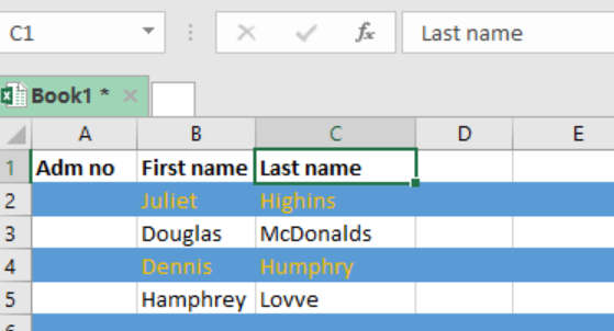
How to Apply Conditional Formatting to an Entire Row
This tutorial shows the reader how they can apply conditional formatting to an entire row. It illustrates how to set up the data, establish your criteria, and name your desired formatting for the rows that are a match. There are examples and illustrations to help you learn.
Highlight Top Values
If you are reporting results in Excel, it might be more impactful if you can highlight the top values or those that are over a certain figure. This piece shows how to accomplish this using conditional formatting. Specifically, you can highlight the top (or bottom) values any color you choose.
How to Lookup an Entire Row in Excel
When working with a large amount of data in Excel, you might need to look up an entire row that matches certain criteria. This tutorial shows how to accomplish this by using the INDEX and MATCH functions. It gives the syntax of the formula, shows how to set up the data, and then provides an example with illustrations on looking up an entire row in Excel.
Highlight Rows with Blank Cells
You might have an Excel spreadsheet and need to identify any blank cells. This is a step-by-step guide that shows how to use conditional formatting to highlight rows that contain blank cells. It uses the function COUNTBLANK, and the end result will be to highlight all the rows that contain blank cells. There are examples and illustrations to follow.
Learn How to Remove Conditional Formatting
If you have an Excel spreadsheet with conditional formatting, there might be some instances where you want to remove or delete. This tutorial walks the reader through the various ways of identifying and then removing conditional formatting from an Excel sheet. There are examples and illustrations throughout.

Find out the ways you can remove conditional formatting in Excel.
Conditional Formatting Highlight Target Percentage
Conditional formatting rules can be used to create various targets and then highlight those targets different colors. This tutorial shows the reader how to create percentage targets in Excel and then use conditional formatting to highlight target percentages in a spreadsheet.
How to Use Excel’s SUMPRODUCT Function
This high-level tutorial explains the SUMPRODUCT function in Excel and its use for multiplying various arrays. It also provides the syntax for the function, some notes for its use, and walks through several examples of using SUMPRODUCT in an Excel sheet.
How to Highlight the 3 Smallest Values with Criteria in Excel
Conditional formatting allows you to choose your conditions or criteria and then apply different formatting, such as bolding, shading, or coloring a cell. This tutorial shows the reader how to highlight the three smallest values in a row or column with examples and illustrations.
Highlight Multiples of Specific Value
This step by step tutorial illustrates how to change the formatting of cells based on a condition. Specifically, it teaches the reader to how Excel can identify multiples of a specified value and then highlight them accordingly.
Conditional Formatting Based on Another Cell
You can apply conditional formatting based on another cell, such as highlighting all values that are above or below the mean or median for a given period. This tutorial shows how to set up this type of conditional formatting with a step-by-step guide that includes examples and illustrations.
Learn how to apply conditional formatting based on another cell with this guide.
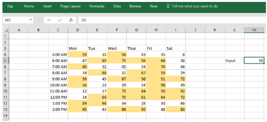
Using Conditional Formatting Times in Excel
Conditional formatting can apply to text, numbers, dates, and times. This tutorial shows the reader how to use conditional formatting with times in Excel. For example, it illustrates how to highlight employees that fall outside normal working parameters, such as clock in and clock out times and total hourly work times.
Highlight Cells that Begin With
When applying conditional formatting to text, you don’t have to have an exact match. This tutorial shows how you can use conditional formatting to highlight cells in Excel with text that begins with your criteria. There are examples and illustrations to follow.
How to Highlight a Row and Column Intersection with Exact Match in Excel
Conditional formatting allows you to highlight an intersecting row and column in Excel that match your criteria. This tutorial shows how to use the OR function to accomplish this.
Working with a Pivot Table that Has Conditional Formatting
If you want to enhance the format and layout of a pivot table, you may be able to use conditional formatting. While there are some restrictions to its use, this guide explains how you can and can’t apply conditional formatting to pivot tables in Excel.
Didn’t find what you need on this list or have another question about Excel? Our Excel experts are standing by to help through a live chat. Your first session is always free. Get started now.


Leave a Comment