How to Apply Conditional Formatting to Blank Cells

We can use the conditional formatting approach for “cells that do not contain any value or for blank cells”. This step by step tutorial will assist all levels of Excel users on how to apply conditional formatting to blank cells.

Apply conditional formatting to blank cells

The aim of this exercise is apply formatting to the cells in Excel that are blank. For example, in Figure 1, the final result is to have all of the blank cells highlighted yellow. Here is how you can accomplish this:

Figure 1 – Final result

Setting up the Data

• First, we will set up our data by inputting the values for the items in the cells we choose.
• Our data is shown below.

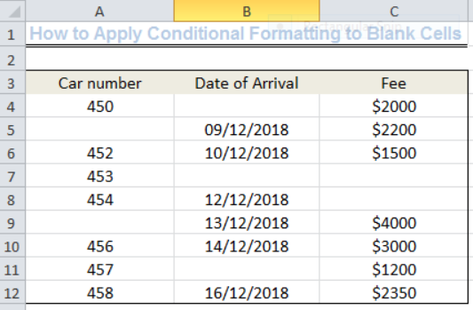Figure 2- Setting up the Data

How to Apply Conditional Formatting To Blank Cells Only

We can see from our data in Figure 1 that the following cells are blank:

• A5 , A9, B4, B7, B11, C7 and C8

We can apply conditional formatting to all of these blank cells to show certain colors, patterns, etc. We can do this by following the simple steps outlined below.

• First, we have to select the data range of interest. The data range is from Cell A4 to Cell C12.
• Next, we have to click on conditional formatting as shown in figure 2 and click on the drop-down arrow.

Figure 3- How to Apply Conditional Formatting for Only Blank Cells

After we have clicked on the drop-down arrow, we will see a New Rule. Click on the New Rule and a dialog box called New formatting Rule will show up as shown in Figure 3.

Figure 4- How to Apply Conditional Formatting for Only Blank Cells

• Where you see Select a Rule Type as shown in Figure 3, click on Format only cells that contain.
• We also need to change the Rule Description to format only cells with blanks by clicking the drop-down arrow.
• We can use a range of conditional formatting options for the blank cells by clicking on Format adjacent to the No Format Set. For this example, let us use the Yellow color to fill cells that are blank. We will click on OK after selecting our choice.

Figure 5- How to Apply Conditional Formatting for Only Blank Cells

As we can see from Figure 5, all of the blank cells are now conditionally formatted in Yellow color.

Figure 6- Output Showing the Result of Conditionally Formatted Blank Cells

How to Apply Conditional Formatting Using a Custom Formula

• Syntax

=ISBLANK(VALUE)

• Syntax

=LEN(VALUE)

Explanation of formulas

A blank cell can contain a character such as space (just like the spaces we give when typing). We will type a space character into one of the blank cells (Cell A9).

The ISBLANK function returns as TRUE when a cell doesn’t contain “anything” and as FALSE when a cell contains at least one character.

The LEN function returns as TRUE for blank cells without any character and FALSE for cells with a character.

When using a custom formula for conditional formatting, it is essential that we enter the formula relative to the active cell in the selection. In this case, the cell is Cell A4. This will automatically update across the range where conditional formatting is intended to be applied.

Still applying the steps above, in figure 3, we will click on Use a formula to determine which cells to format.

Figure 7- How to Use a Custom Formula for Conditional Formatting

We will click on OK afterward with the result being Figure 7. Remember that Cell A9 IS NO LONGER EMPTY BUT CONTAINS A SPACE CHARACTER.

Figure 8 – Output Showing the Result of Conditional Formatting with a Custom Formula

Using the same approach, we can input this string =LEN(A4)=0 into the Rule Description of figure 6 and we will arrive with the same result as figure 7.

How to Conditionally Format a Column Based on the Result from another Column

We can conditionally format the car number column based on the presence of a blank or visually empty cell (cell with at least a character). Cell A9 is visually empty because it has a space character. To do this, we can use the string below:

=$B4=””

We will select the car number column range (Cell A4 to Cell A12), follow the same procedure, and just like figure 6, we will input the string.

=$B4=””

The result in Figure 8 shows that cells in Column A have been conditionally formatted if they have corresponding cells on Column B (Date of Arrival) that are blank.

Figure 9- Output of Conditional Formatting Based on the Blank Cells in Column B

If you are having any difficulty applying this, we have experts who are willing to help.

Are you still looking for help with Conditional Formatting? View our comprehensive round-up of Conditional Formatting tutorials here.