Highlight top values

Reporting insights from data often requires to highlight values based on criteria. One of the most common uses is to highlight top or bottom values. Excel offers some great ways to highlight values. We can highlight top values using conditional formatting in Excel. In this tutorial, we will learn how to highlight top values in Excel.

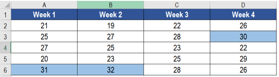Figure 1. Example of How to Highlight Top Values in Excel

Generic Formula

=A2>LARGE(data,N)

How the Formula Works

We use the LARGE function in this formula. It returns the nth largest value from an array or range. The first argument is this range and the second one is the value “n”. Large returns the nth largest value in the date. Afterwards, the formula compares every other value with the nth largest value. We are using the greater than or equal to operator (>=) to perform this comparison. Any cell having a value greater than or equal to this nth largest value returns TRUE, others return FALSE. The TRUE values triggers the rule, thus the conditional formatting is applied.

Setting up Data

The following example uses a temperature database for January 2019. Column A to D has these temperatures.

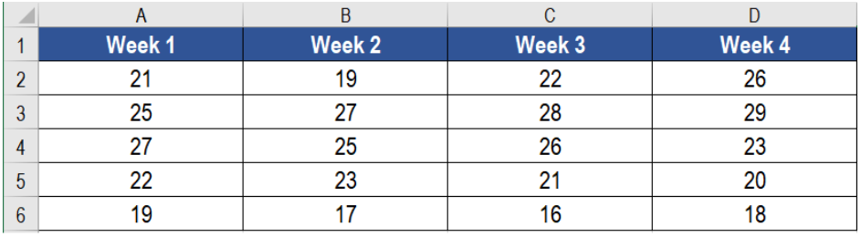Figure 2. The Sample Data Set

To highlight the top three temperature values, we need to

• Select cells A2 to D6.
• From the home tab in the ribbon, go to Conditional Formatting. Next, we need to click on New Rule.

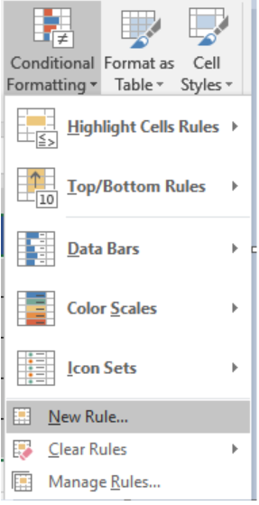Figure 3. Example of how to Apply Conditional Formatting

• Select Use a formula to determine which cells to format.

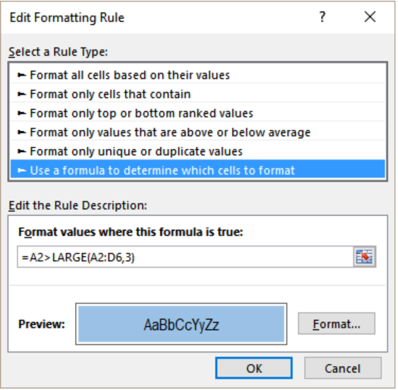Figure 4. Applying the Formula to the Conditional Format

• Click the Format values where this formula is true box. On the formula box, assign the formula =A2>LARGE(A2:D6,3).  
• Click the Format tab near the preview box.
• Next, we need to go to  Fill>Background Color and select the color we want to highlight in.  

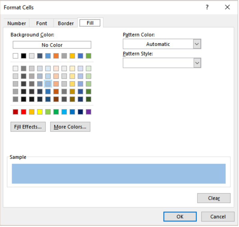Figure 5. Setting the Display Options

• Click OK twice.

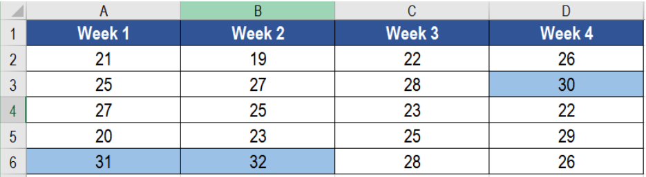Figure 6. The Final Result

This will highlight the top 3 values in columns A to D.

Most of the time, the problem you will need to solve will be more complex than a simple application of a formula or function. If you want to save hours of research and frustration, try our live Excelchat service! Our Excel Experts are available 24/7 to answer any Excel question you may have. We guarantee a connection within 30 seconds and a customized solution within 20 minutes.

Are you still looking for help with Conditional Formatting? View our comprehensive round-up of Conditional Formatting tutorials here.