

Conditional Formatting is a feature in Excel that allows us to change the format of cells based on a set of rules or conditions. This step by step tutorial will assist all levels of Excel users in applying conditional formatting to highlight multiples of a specific value.
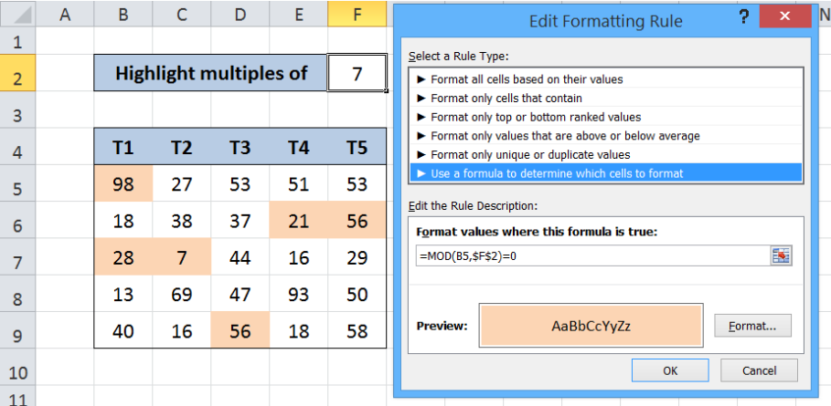 Figure 1. Final result: Highlight multiples of specific value
Working formula: =MOD(B5,$F$2)=0
Syntax of MOD Function
MOD function returns the remainder after dividing a number by a divisor; the result of MOD always follows the sign of the divisor
=MOD(number, divisor)
- number – the number for which we want to divide by a divisor and find the remainder
- divisor – the number by which we want to divide number
Setting up the Data
Our data consists of five columns from column B to F, with each column containing five numbers. In cell F2, we enter our criteria which is the number 7, whose multiples we want to highlight in our data. We want to use conditional formatting to highlight the values which are multiples of the number 7.
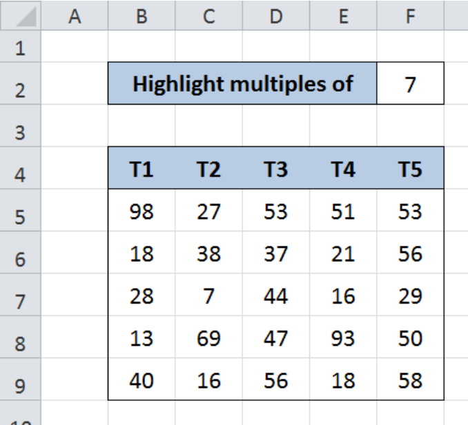 Figure 2. Sample data for conditional formatting based on another cell’s value
Highlight multiples of 7
We want to highlight the cells in the range B5:F9 containing values that are multiples of 7. We can do this through conditional formatting and the MOD function by following these steps:
Step 1. Select the cells we want to highlight. In this case, select cells B5:F9.
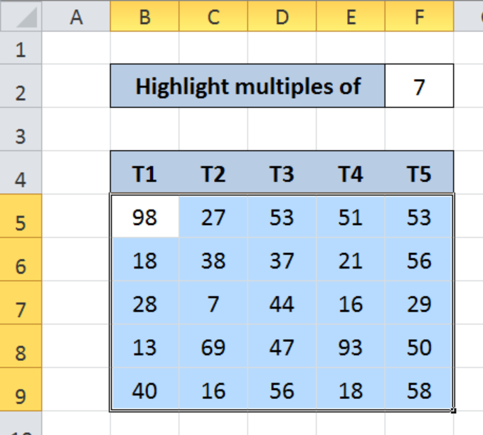 Figure 3. Selection of the data range for conditional formatting
Step 2. Click the Home tab, then the Conditional Formatting Menu and select “New Rule”.
The New Formatting Rule dialog box will pop up.
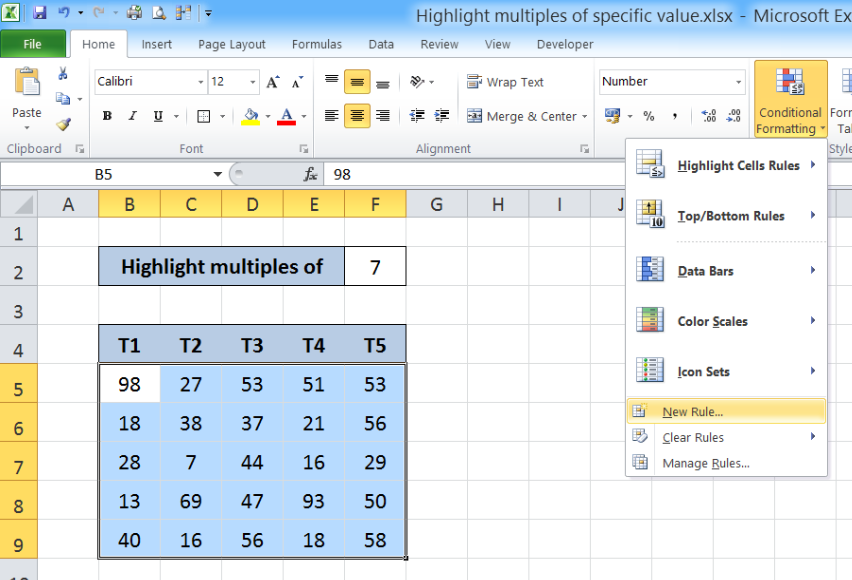 Figure 4. Creation of a new rule in conditional formatting
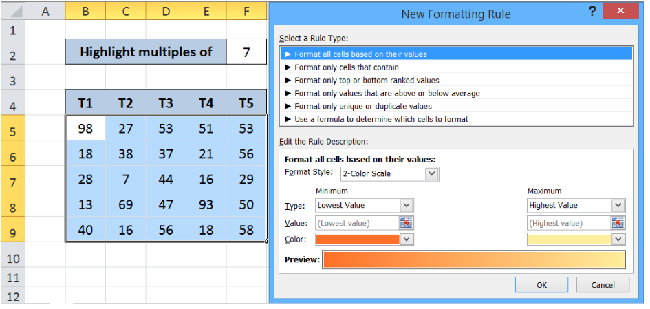 Figure 5. New Formatting Rule preview
Step 3. Select the Rule Type “Use a formula to determine which cells to format” and enter this formula in the dialog box :
=MOD(B5,$F$2)=0
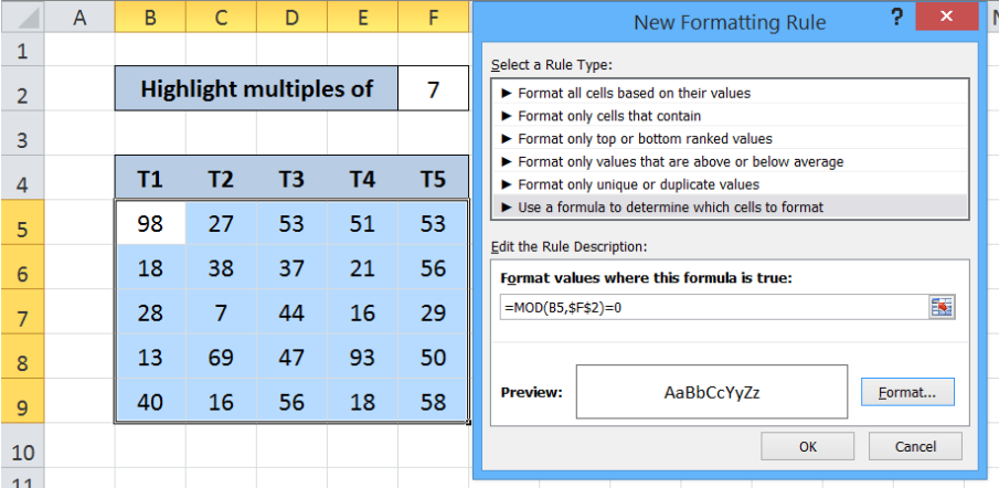 Figure 6. Entering the formula as a condition or formatting rule
Our formula serves as the condition or rule that will trigger the conditional formatting. Each cell in B5:F9 will be divided by F2 or “7”, and the MOD function will return the remainder. If the remainder is equal to zero “0”, the value in that cell is a multiple of 7 and the format will be changed.
The dollar sign “$” fixes cell F2 to enable our formula to work properly across all cells in B5:F9.
To change the format, let us proceed to the next step.
Step 4. Click “Format” and then decide on the new format to apply to the cells in B5:F9. We can change the font, borders or fill the cells with different colors.
Example
Select “Fill” and choose Orange, Accent 6, Lighter 60% and click OK.
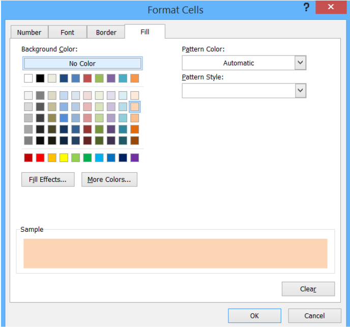 Figure 7. Selection of the format to use
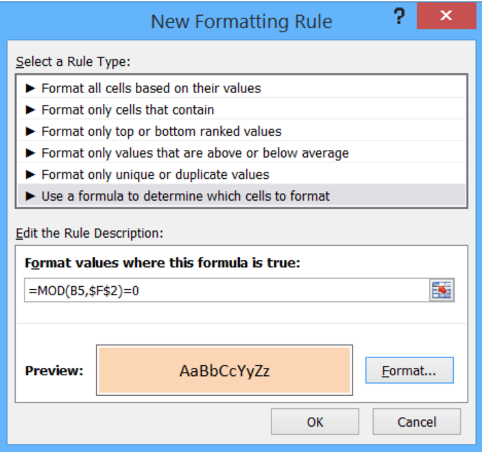 Figure 8. Completion of the new formatting rule with formula and selected format
This rule highlights the cells that are multiples of 7. As a result, cells B5, B7, C7, D9, E6 and F6 are highlighted as shown below.
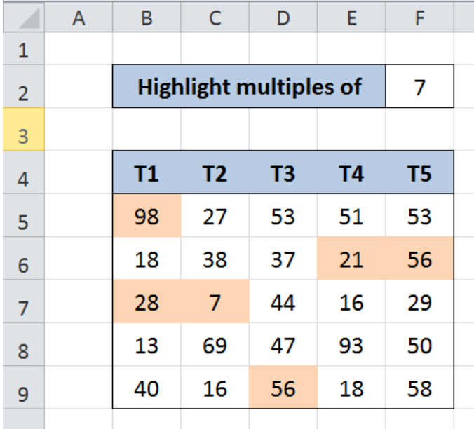 Figure 9. Output:Highlight multiples of 7 using conditional formatting
With conditional formatting and the MOD function, we are able to highlight multiples of 7. With our formula, we can easily highlight multiples of other numbers by simply changing the value of F2.
Most of the time, the problem you will need to solve will be more complex than a simple application of a formula or function. If you want to save hours of research and frustration, try our live Excelchat service! Our Excel Experts are available 24/7 to answer any Excel question you may have. We guarantee a connection within 30 seconds and a customized solution within 20 minutes.


Leave a Comment