

Conditional Formatting is a feature in Excel that allows us to change the format of cells based on a set of rules or conditions. This step by step tutorial will assist all levels of Excel users in applying conditional formatting to highlight dates falling in the next N days.
 Figure 1. Final result: Highlight dates in the next N days
Working formula: =AND(B5>TODAY(),B5<=(TODAY()+$E$2))
Syntax of AND Function
AND function evaluates all logical tests and returns TRUE if all arguments are TRUE; FALSE if one or more arguments is FALSE
=AND(logical1, [logical2], ...)
- logical1– the first condition that we want to test
- only logical1 is required; succeeding logical conditions are optional
Syntax of TODAY Function
TODAY function returns the current date
=TODAY()
- TODAY function does not have any arguments
- It can be used in combination with other functions and mathematical operations to obtain the desired results
Setting up the Data
Our data consists of four columns from column B to E, with each column containing five dates. In cell F2, we enter the number “30” which serves as our criteria. We want to use conditional formatting to highlight dates that fall in the next 30 days from today.
 Figure 2. Sample data: Highlight dates in the next 30 days
Supposing the date today is January 29, 2019, then the date 30 days from today would be February 28, 2019. Hence, we want to highlight the dates in between January 29, 2019 and February 28, 2019.
Highlight dates in the next 30 days
We want to highlight the cells in the range B4:F9 containing the dates that fall in the next 30 days from today. We can do this through conditional formatting and the functions AND and TODAY by following these steps:
Step 1. Select the cells we want to highlight. In this case, select cells B5:E9.
 Figure 3. Selection of the data range for conditional formatting
Step 2. Click the Home tab, then the Conditional Formatting Menu and select “New Rule”.
The New Formatting Rule dialog box will pop up.
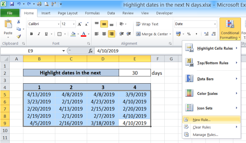 Figure 4. Creation of a new rule in conditional formatting
 Figure 5. New Formatting Rule preview
Step 3. Select the Rule Type “Use a formula to determine which cells to format” and enter this formula in the dialog box :
=AND(B5>TODAY(),B5<=(TODAY()+$E$2))
The dollar sign “$” fixes cell E2 which serves as our criteria, to enable our formula to work properly across all cells in B5:E9.
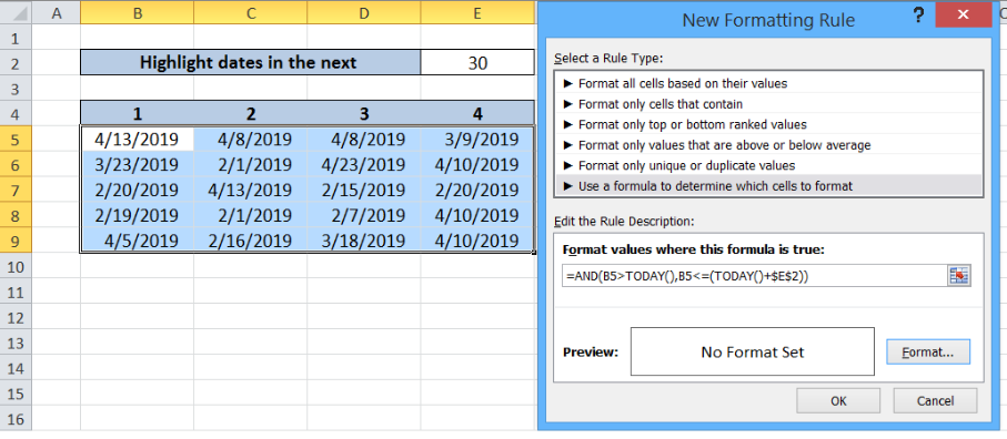 Figure 6. Entering the formula as a condition or formatting rule
Our AND formula contains two criteria. First, it evaluates if the date in B5 is greater than the date today. Next, it evaluates if the date in B5 is less than or equal to the date 30 days from today, as given by the formula TODAY()+30.
Excel stores dates as serial numbers, making it possible to perform calculations involving dates. In this example, we refer to the date today as January 29, 2019, while the date 30 days from now would be February 28, 2019.
Hence, for every date in the range B5:E9 that falls between January 29, 2019 and February 28, 2019, the format will be changed.
To change the format, let us proceed to the next step.
Step 4. Click “Format” and then decide on the new format to apply to the cells in B5:E9. We can change the font, borders or fill the cells with different colors.
Example
Select “Fill” and choose Orange, Accent 6, Lighter 60% and click OK.
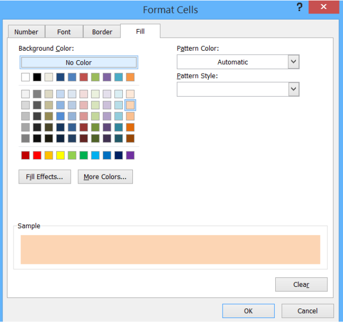 Figure 7. Selection of the format to use
 Figure 8. Completion of the new formatting rule with formula and selected format
This rule highlights the cells that fall in the next 30 days from today. As a result, cells B7, B8, C6, C8, C9, D7, D8 and E7 are highlighted as shown below.
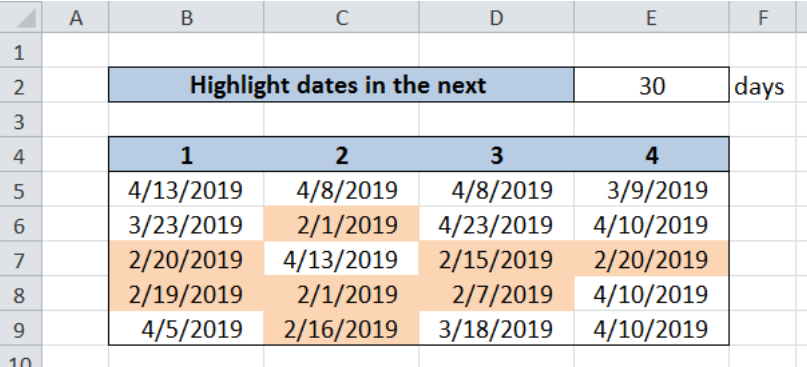 Figure 9. Output: Highlight dates in the next 30 days
Using conditional formatting with the AND and TODAY functions, we are able to highlight dates that fall in the next 30 days. With our formula, we can easily highlight our desired dates by simply changing the value of F2.
Most of the time, the problem you will need to solve will be more complex than a simple application of a formula or function. If you want to save hours of research and frustration, try our live Excelchat service! Our Excel Experts are available 24/7 to answer any Excel question you may have. We guarantee a connection within 30 seconds and a customized solution within 20 minutes.


Leave a Comment