

The conditional formatting is used to create visual differentiation in a large set of data, in some standard format. Normally, the data can be visually differentiated using one or more rules, however, in this article, we will discuss how to apply conditional formatting with 2 conditions.
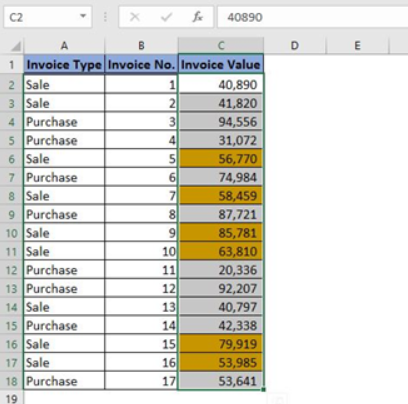
Figure 1 – Final result
1 Column, 2 Rules, 2 Conditions
Let’s assume that we have a set of different Sales Invoice data and we want to segregate invoices using conditional formatting which are either below or above $50,000. In order to achieve this, we need to follow the below steps:
- Select the data range containing the invoice values, click on “Conditional Formatting” available on “Home” tab.
- Choose “New Rule” from the drop-down menu.
- Choose the rule type “Format only cells that contain”. In the “Format only cells with” section, select “Cell Value” in the first drop-down box and “greater than” from the second drop down. Write 50000 in the value field.
- Click “Format” to display the Format Cells dialog box, choose the format as per your liking. (Figure 2)
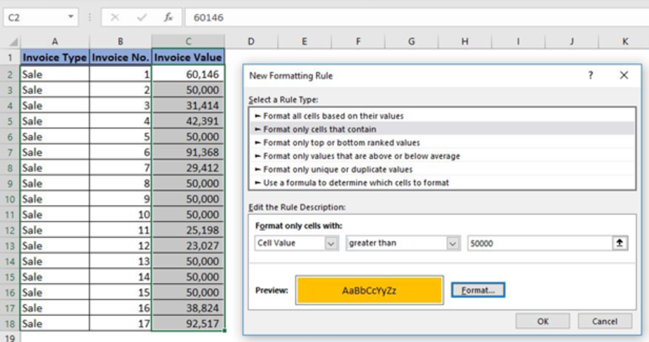 Figure 2 – Selection and application of the first condition
- Click “OK” for the formatting to come into effect.
- After completing the above steps, the invoices having a value greater the $50,000 will be highlighted. (Figure 3)
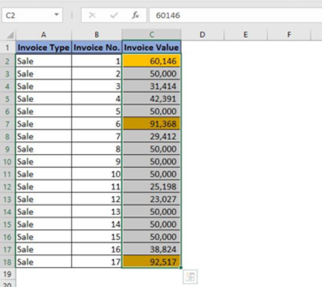 Figure 3 – Result after application of the first condition
- We have applied the first condition, now, we will move on to the application of the second condition.
- The initial steps involved are exactly the same. We will again select the data range containing the invoice values then go to “Home>Conditional Formatting>New rule”
- Choose the rule type “Format only cells that contain”. In the “Format only cells with” section, select “Cell Value” in the first drop-down box and “less than” from the second drop down. Write 50000 in the value field.
- Click “Format” to display the Format Cells dialog box, choose the format as per your liking. (Figure 4)
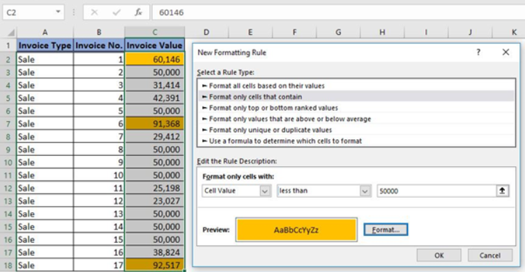 Figure 4 – Selection and application of the second condition
- Click “OK” for the formatting to come into effect.
- The final result will be the highlighted invoice values that are either greater or lower than $50,000. (Figure 5)
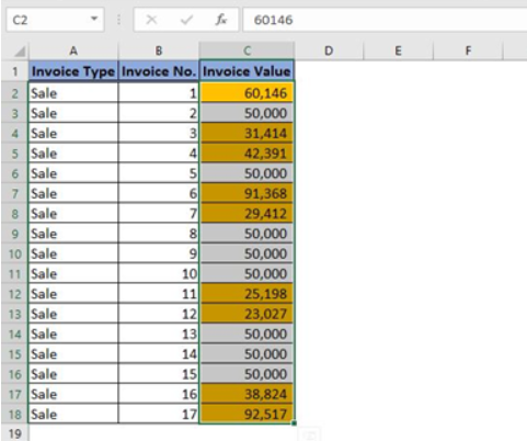 Figure 5 – Final Result after application of 2 Conditions
- We can also view the rules that we have applied on our dataset by going to “Home>Conditional Formatting>Manage Rules”. (Figure 6)
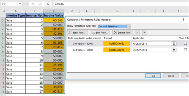 Figure 6 – Rules showing 2 conditions applied to the same dataset
1 Column, 1 Rule, 2 Conditions
The second way through which we can apply two conditions on the same dataset is by using a formula. In this technique, the steps involved are as follows:
- Select the data range containing the invoice values.
- We will reach to the conditional formatting dialog box in the usual way i.e. “Home>Conditional Formatting>New rule”.
- Now instead of selecting rule type “Format only cells that contain”, we will select “Use a formula to determine which cells to format”.
- The formula that we will apply, to select our invoices that have a value of greater or lower than $50,000, is
=OR(C2>50000,C2<50000) - Click “Format” to display the Format Cells dialog box, choose the format as per your liking. (Figure 7)
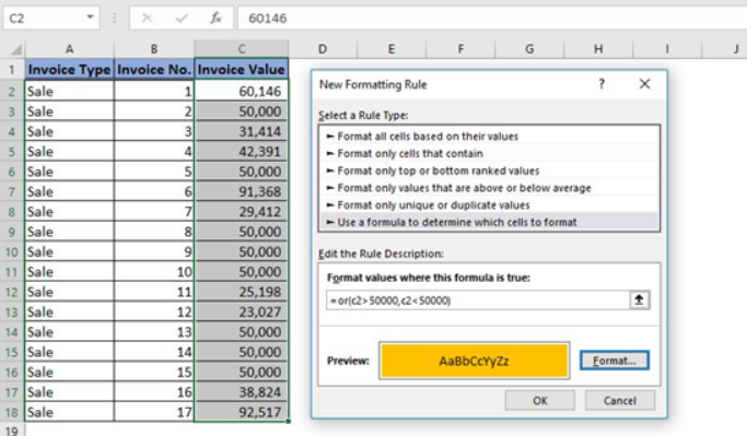 Figure 7 – Application of formula to cater 2 conditions in 1 rule
In the above formula we have used “OR” operator to test two conditions to identify invoices having value either greater or lower than $50,000. After application of formatting rules click “OK”. We will see the same results which we saw in the first technique. (Figure 8)
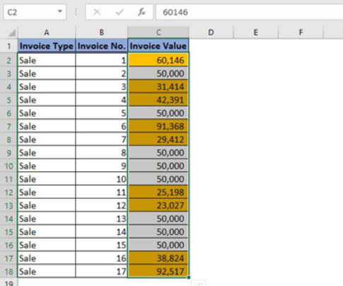 Figure 8 – Result after application of conditional formatting using a formula
In the above scenario, the “Manage Rules” dialog box will show one rule applied to the dataset with two conditions. (Figure 9)
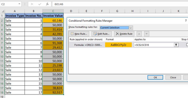 Figure 9 – Rules Manager showing only one rule
2 Columns, 1 Rule, 2 Conditions
Up till now, we were applying 2 conditions on a single column but what if we wanted to apply 2 conditions on separate columns? Well, we will look at the solution to this problem now. As a start, let’s change our sales data to include purchase as well. (Figure 10)
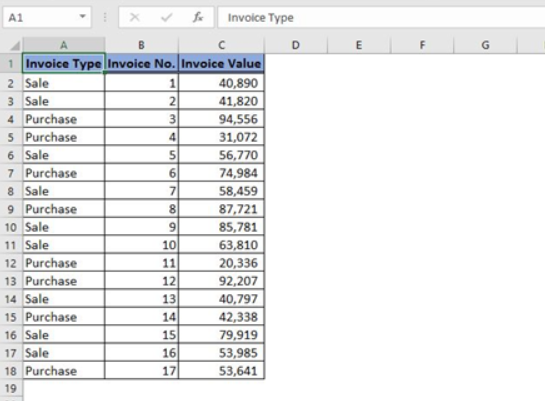 Figure 10 – Data for purchase and sale
In the above data, we will highlight only those values that are greater the $50,000 and pertain only to sales. To achieve this, we will do the following:
- Select the data range containing the invoice values.
- Go to the conditional formatting dialog box. “Home>Conditional Formatting>New rule”.
- Select “Use a formula to determine which cells to format”. The formula that we will apply, to select our invoices that have a value of greater than $50,000 and pertain only to sales, is =AND(A2=“Sale”,C2>50000).
- Click “Format” to display the Format Cells dialog box, choose the format as per your liking. (Figure 11)
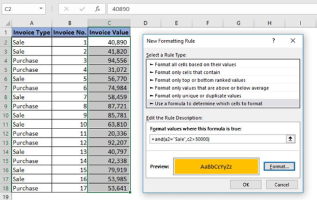 Figure 11 – Application of 2 conditions on separate columns
In the above formula, we have used “AND” operator to test two conditions to identify sales invoices having a value greater than $50,000. After application of formatting rules click “OK”. The final result will be highlighted sales invoices having a value greater than $50,000. (Figure 12)
Figure 12 – Final result of the application of testing two conditions on separate columns
Instant Connection to an Expert through our Excelchat Service
Most of the time, the problem you will need to solve will be more complex than a simple application of a formula or function. If you want to save hours of research and frustration, try our live Excelchat service! Our Excel Experts are available 24/7 to answer any Excel question you may have. We guarantee a connection within 30 seconds and a customized solution within 20 minutes.


Leave a Comment