

How to use SUMIF in Google Sheets
SUMIF has two parts, SUM and IF. If a range of cells meets the condition, then this function sums the numbers related to that condition. The syntax of SUMIF function in Google Sheets is same as the Excel syntax;
=SUMIF(range, criterion, [sum_range])
Where,
range: It is a cells range that is tested against a criterion
criterion: It is a condition to be met. It can contain a value (number, text, date), expression, logical operator, wildcard character, cell reference or another function.
sum_range: It is a cell range to sum the numbers where a condition is met.
Rules for SUMIF
There are some rules to follow while using SUMIF function correctly;
- SUMIF function is not case-sensitive.
- Size of range and sum_range must be equal
- range and sum_range could be the same if a numeric range is tested against a number as the criterion.
- If criterion contains a text, date, expression, logical operator and wildcard, then it must be enclosed in double quotation marks, such as “t-shirt”, “>5”, “*”
- If the criterion is a number, cell reference or another function, then it must not be enclosed in double quotation marks such as B1 or Today()
- If criterion contains both logical operator and cell reference or another function, then they must be joined together by using an ampersand (&), such as “>”&B2, or “>”&Today()
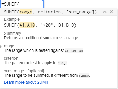
When you enter SUMIF function in Google Sheets, an auto-suggest box pops up, containing syntax, example, summary related to SUMIF function and explanation of each part of function as shown below.
In this article, you will learn how to use SUMIF function in Google Sheets in different criterion cases with examples.
SUMIF function with Text criteria
If you want to sum the numbers in cells range that have a specific text value in a parallel cells range, another column and same row, supplied as criteria.
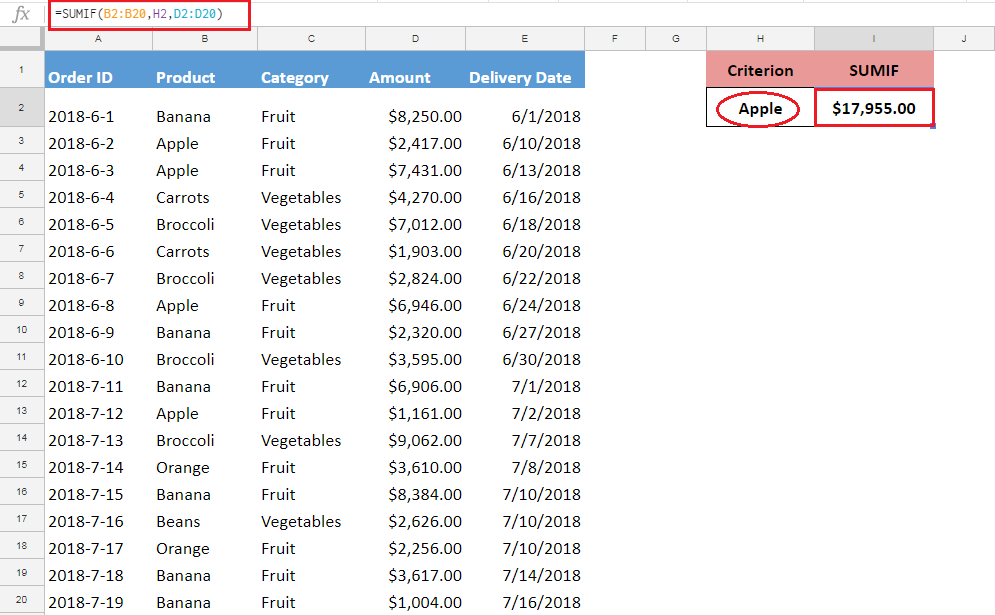
For example, you have a data set of sales order information for various products, and you want to sum the amounts of orders for “Apple” product as the criterion. So the criterion can be supplied in SUMIF function as text value in double quotation marks or as cell reference without double quotation marks, such as;
=SUMIF(B2:B20,"Apple",D2:D20)
OR
=SUMIF(B2:B20,H2,D2:D20)
Here,
B2:B20 is the range of cells
“Apple” or H2 is the criterion as a text value or cell reference
D2:D20 is sum_range of cells

SUMIF function with Number criteria
If you want to sum the numbers that meet certain criterion as specified in SUMIF function in Google Sheets, by using comparison operators, like greater than (>), less than (<), greater than equal to (>=), less than equal to (<=) or Not equal to (<>).
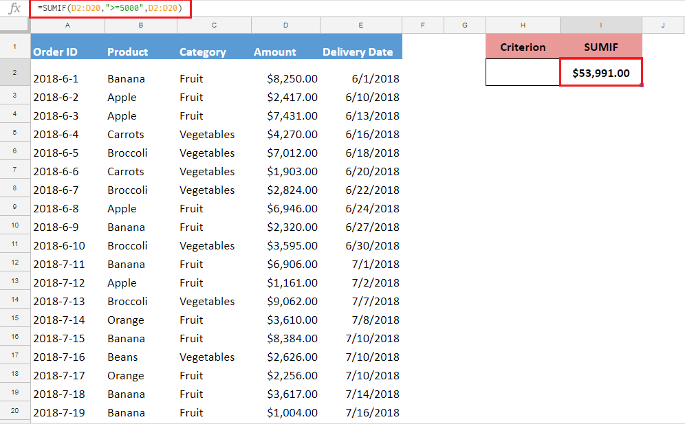
Suppose you want to sum all order amounts that are greater than equal to $5,000. In this case, the range and sum_range are the same, as order amounts are listed in the same range and criteria are also applied on the same range. In this case, the SUMIF function can be applied in one of these ways;
=SUMIF(D2:D20,">=5000",D2:D20)
OR
=SUMIF(D2:D20,">="&H2,D2:D20)
As you can see criterion expression is supplied in double quotation marks in SUMIF function, such as “>=5000”, but if the criterion is supplied as expression and cell reference, then they are joined together by an ampersand (&), such as “>=”&H2.

SUMIF function with Date criteria
You can sum the numbers based on date criteria by using any of the comparison operators. The date must be supplied in double quotation marks in a format that is understandable by Google Sheets, or date must be supplied as cell reference without double quotation marks, or date must be supplied using a date function like DATE() or TODAY().
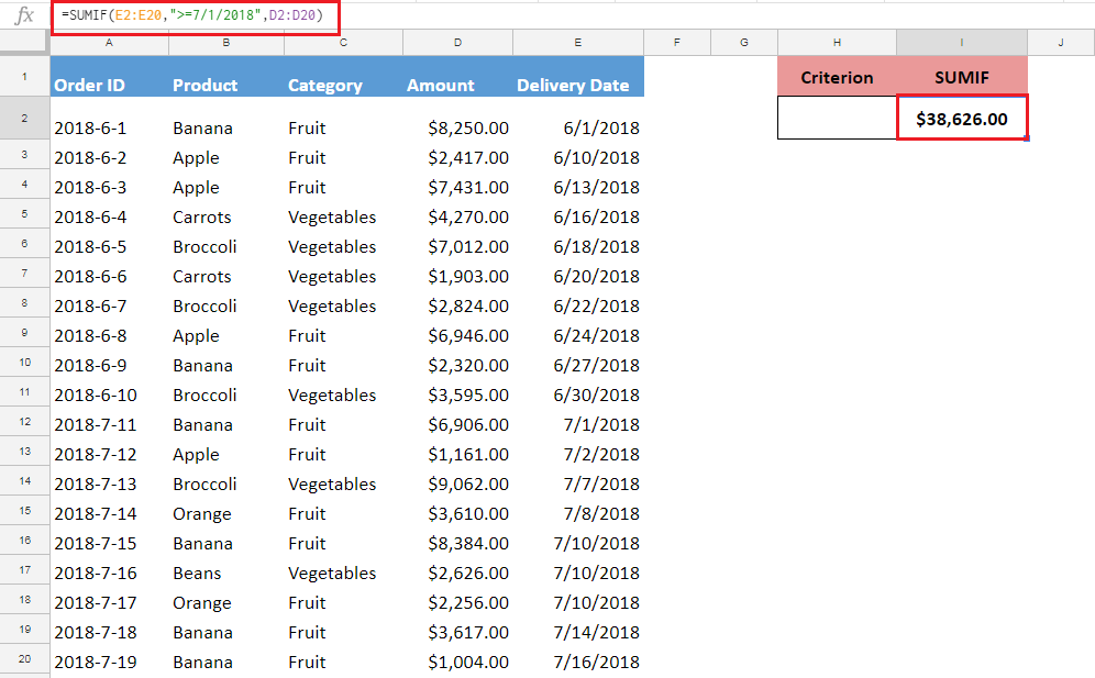
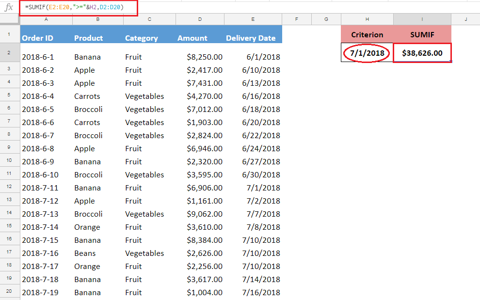
Suppose you want to sum the order amounts that are greater than equal to (>=) a criterion date, say 7/1/2018, so you can sum those amounts using SUMIF function in any of the following ways;
=SUMIF(E2:E20,">=7/1/2018",D2:D20)
OR
=SUMIF(E2:E20,">="&H2,D2:D20)
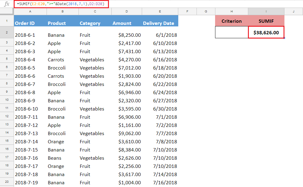
OR
=SUMIF(E2:E20,">="&Date(2018,7,1),D2:D20)
SUMIF function with Blank or Non-Blank cells criteria
You can sum the numbers, based on criteria where cells are blank or non-blank in a range of cells using SUMIF function in Google Sheets.
Suppose in your data set some of the orders do not have delivery date mentioned, so you want to sum the order amounts based on criteria where delivery date is mentioned (non-blank), and where delivery date is not mentioned (blank).
- SUMIF function with Blank cells criteriaThis SUMIF formula will sum the order amounts where delivery date is not mentioned in range. Criterion is supplied as double quotation marks without any space in-between, such as “”.
=SUMIF(E2:E20,"",D2:D20)![]()
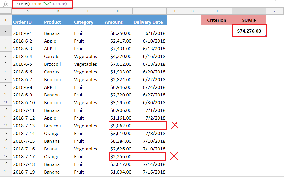
- SUMIF function with Non-Blank cells criteriaThis SUMIF formula will sum the order amounts where delivery date is mentioned in range. Criterion is supplied by using comparison operator Not Equal to (<>) in double quotation marks, such as “<>”, means where cells are not blank. This excludes those amounts where delivery dates are blank.
=SUMIF(E2:E20,"<>",D2:D20)![]()

Still need some help with Excel formatting or have other questions about Excel? Connect with a live Excel expert here for some 1 on 1 help. Your first session is always free.


Leave a Comment