

While analyzing data in Excel, you might need to calculate averages of different subsets of a specified data range to get the variations or fluctuations in the data. If you want to forecast the trend in data, this is referred to as a moving average, rolling average, running average, or moving mean.
Finding the Rolling Average in Excel
This technique is used to analyze the trend in data for a certain interval of time or period. It is frequently used to get the trends in sales data, economic data, statistical data, weather temperatures, and stock prices to show the average value of data set over a given period of time. For example, you need to calculate the moving average of sales data for the last 3 months to get the trend in sales data.
In this article, you will learn how to calculate moving average or rolling average in Excel. In Excel, there are various methods to calculate moving average or rolling average which will be discussed here.
Suppose you have business sales data of 12 months and you want to see the trend in sales by calculating a moving average or rolling average over a period of the last 3 months. You can calculate the moving average by using the following methods in Excel.
Using the AVERAGE function in Excel
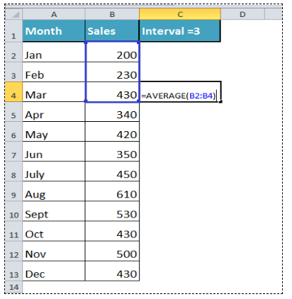
Using the Average function, you can easily calculate a series of averages or a moving average of the required interval of time/period of a given data range of 12 months sales. As you need to get the series moving averages of the last 3 months, therefore you need to enter the cell references of first three cells in the AVERAGE function in the third adjacent cell of monthly sales data, like in cell C4, and drag or copy it down, as shown below.
=AVERAGE(B2:B4)
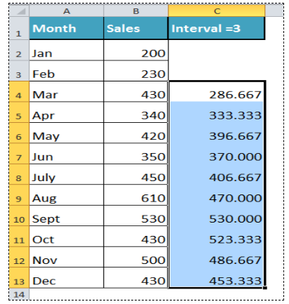
In column C, you get a series of averages for a period of last 3 months, and that is referred to as moving the average or rolling average of last 3 months sales data.
Using Analysis ToolPak Add-in for Moving Average in Excel
In Excel, Analysis ToolPak add-in has a built-in option to calculate moving average for the range of data. For this purpose, you need to first install this add-in from available add-ins in Excel Options dialog box.
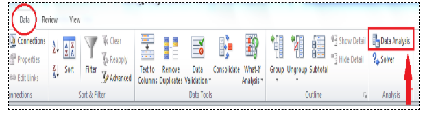
After installing Analysis ToolPak add-in, you need to go back to the main Excel interface, click on the Data tab and click on Data Analysis button in Analysis section.
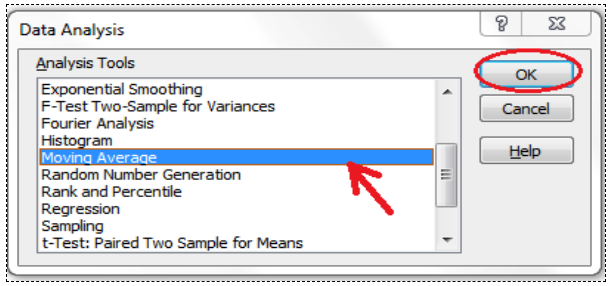
A Data Analysis dialog box appears, click on Moving Average option from Analysis Tools and click on OK.
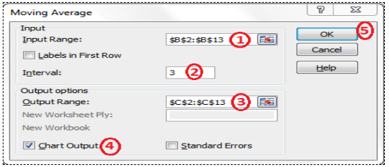
Now, Moving Analysis dialog box appears to make calculations. You need to do followings in this dialog box;
- First, put a cursor in the Input Range section and select the range of sales data B2:B13.
- Second, go to Interval section and insert 3 as an interval period.
- Third, insert the data range to show the result of the moving average in the Output Range section as C2:C13.
- Fourth, you can select Chart Output checkbox optionally to generate chart as well showing a trend of sales.
- Finally, press OK button to calculate the moving average of sales data for the last 3 months.
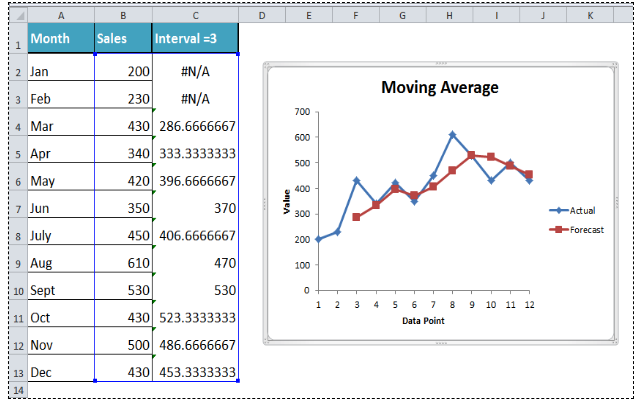
You will get a series of moving averages in output cells range, and a Moving Average chart will also be created, showing actual and forecast trend based on the last 3 months sales figures.
Adding Moving Average Trendline in an Excel Chart
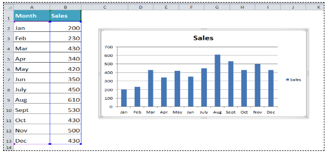
You can show Moving Average Trendline in an existing chart in Excel by supplying interval as 3 months in our example here. First, you need to insert a Column Chart for 12 months sales figures in Excel, and then you need to add Moving Average Trendline in that chart.
First, insert a column Chart for the selected range of data below.
Click anywhere in chart area, in Chart Tools, go to Layout tab, click on the drop-down button of Trendline button in Analysis section and then click on More Trendline Options.
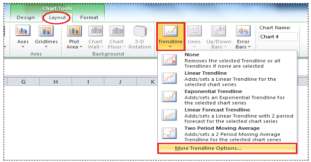
A Format Trendline dialog box appears. In Trendline Options, select Moving Average and enter 3 as period and click the Close button.
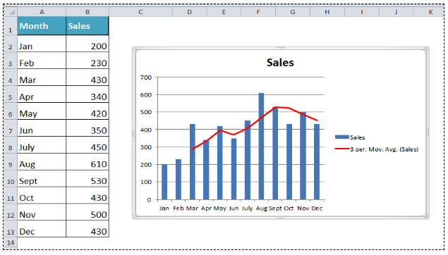
A Moving Average Trendline is added in the created chart showing the monthly sales performance in Excel. This approach is good where you do not need to calculate and show moving average figures, but you only need to show the trend of a sales forecast based on the moving average over a certain period.
Still need some help with Excel formatting or have other questions about Excel? Connect with a live Excel expert here for some 1 on 1 help. Your first session is always free.
Are you still looking for help with the VLOOKUP function? View our comprehensive round-up of VLOOKUP function tutorials here.


help with this calculating average?