If you want to learn how to calculate the average in Excel, AVERAGE and AVERAGEA functions are the answer. The main focus of the article will be on AVERAGE function and difference between AVEREGEA with detailed examples. Some advanced techniques will be also covered including AVERAGEIF and AVERAGEIFS functions. After this tutorial you will be able to calculate: an average of numbers in the range, the average of non-blank cells in range, average based on single or multiple criteria defined – which is very useful knowledge for everyday Excel problem-solving.
1. Calculate Average of Cells
Average of cells containing numbers can be easily calculated using AVERAGE or AVERAGEA functions. AVERAGE function calculates the average of cells in the defined range which contain numbers:
=AVERAGE(range)
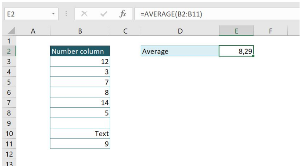
The below example shows how to calculate the average of cells containing numbers in range B2:B11:
=AVERAGE(B2:B11)

As you can see, in our range we have 2 text cells and one blank cell, which does not take in the count when calculating the average. This means that the average is calculated as the sum of number cells divided with their count: 58/7 = 8.29.
On the other side, if we want to calculate the average in defined range taking in the count all cells (numbers, text) which are not blank, then function AVERAGEA should be used. Syntax is the same as for AVERAGE function, so we will use the same example as previous and see what happens:
=AVERAGEA(B2:B11)

If we compare the result to the previous example, we can see it is lower because the sum of numbers is the same, but the count of non-blank cells is greater. In this case, we have 9 non-blank cells, so the average is: 58/9 = 6.44
2. Calculate Average with Criteria
It is often necessary to calculate the average of range with some criteria (for example, the average price of a specific product). For this purpose, AVERAGEIF function is used, which calculates the average for a range based on given criteria. Formula syntax looks like:
=AVERAGEIF(Criteria_range; Criteria; Average_range)
Criteria_range is the range for which we want criteria to be used. Criteria are the value from Criteria_range for which we want to calculate average. Average_range is the range on which average is being calculated. Let’s now look at one example of AVERAGEIF function usage:
=AVERAGEIF(B3:B9;"Bread";C3:C9)

In this example, we want to get the average price (column B is our Average range) of Bread, which is criteria in Criteria range (column B). The average is calculated based on 2 values matching criteria.
Please note that we can put cell reference instead of hardcoded value (in our case “Bread”) so the result will dynamically change based on cell value in criteria. Here is the example of this case:
=AVERAGEIF(B3:B9;F2;C3:C9)

In our criteria, we can also put part of the string for which we want to calculate average. In the following example, we want to calculate the average for all fields containing string “Bread”. To do this, in the criteria we need to put “*Bread*”. Let’s look at the example:
=AVERAGEIF(B3:B10;"*Bread*";C3:C10)

Another very useful example is criteria with logical operations (greater than – “>”, less than – “<”, equal or greater than – “=>”, less than or equal to – “<=”). This possibility is often used when it comes to dealing with numbers, so let’s look at the following example:
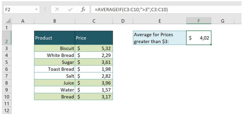
=AVERAGEIF(C3:C10;">3";C3:C10)

In this case, we wanted to calculate the average of all prices that are greater than $3. Column C (Price) is put as Criteria range, and expression “>3” is Criteria. Total of 4 entries was found an average is calculated as 16.06/4 = 4.02.
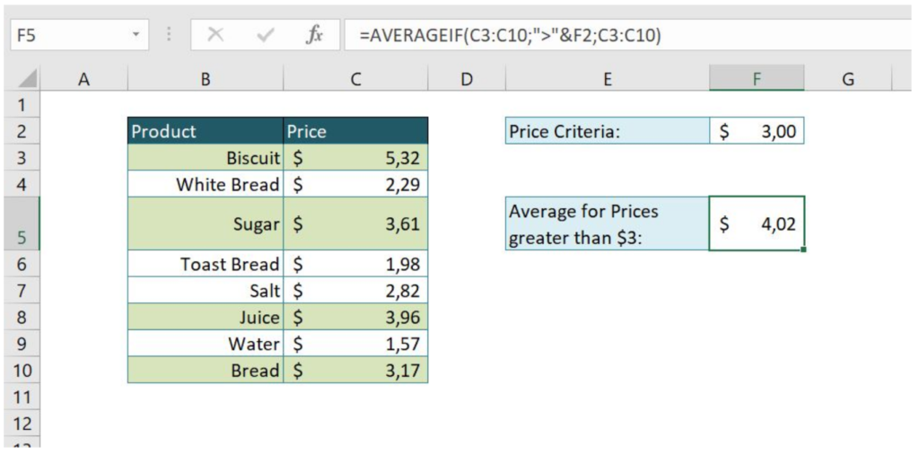
As in the previous example, we can also put reference cell as criteria, instead of hardcoded value “>3” and enable dynamical change of formula result based on entered value. Here is the example:
=AVERAGEIF(C3:C10;">"&F2;C3:C10)

Again we got the same result, but now our criteria are in cell F2. In our function we put logical operation “>” (which means that we want values greater than) and concatenated it using the ampersand (&) with our reference cell F2. Our criteria in function look like “>”&F2.
3. Calculate Average with Multiple Criteria
While going through the previous topic and getting in touch with AVERAGEIF function, you surely wondered if it is possible to combine criteria conditions. The answer is AVERAGEIFS function which calculates the average based on multiple criteria. The syntax of the function looks like:
=AVERAGEIFS(Average_range; Criteria_range1; Criteria1; Criteria_range2; Criteria2; … )
Average_range is the range on which average is being calculated. Criteria_range is the range for which we want criteria to be used. Criteria are valued from Criteria_range for which we want to calculate average. We can put as many criteria as we need. Let’s now look at one example of AVERAGEIFS function usage:
=AVERAGEIFS(C3:C10;B3:B10;F2;C3:C10;">"&F3)

As you can see, two conditions from the previous topic were combined, so we are calculating the average price for all Products containing “Bread” string and all Prices greater than $3. Our Average range is C3:C10 (Price), Criteria range1 is B3:B10 (Products) with Criteria1 in cell F2 (*Bread*), Criteria range2 is C3:C10 (Price), with Criteria2 greater than the value in cell F3 ($3) – “>”&F3. As a result, we have 3 rows containing “Bread” in Products, but only 2 of them have the price greater than 3, so the average is 6.62/2 = 3.31.


Leave a Comment