

When you are analyzing data or making plans for the future, it helps to know several formulas in Excel that will calculate rates of growth. While some are built into the program, you will need the right formulas to get your desired average growth rate.
How to calculate the Compound Average Growth Rate
Annual Average Growth Rate (AAGR) and Compound Average Growth Rate (CAGR) are great tools to predict growth over multiple periods. You can calculate the average annual growth rate in Excel by factoring the present and future value of an investment in terms of the periods per year.
CAGR can be thought of as the growth rate that goes from the beginning investment value up to the ending investment value where you assume that the investment has been compounding over the time period. In this tutorial, you will learn how to calculate the Average Annual Growth Rate and Compound Annual Growth Rate in Excel.
How to calculate the Average Annual Growth Rate
The Average annual growth rate (AAGR) is the average increase of an investment over a period of time. AAGR measures the average rate of return or growth over constant spaced time periods.
To determine the percentage growth for each year, the equation to use is:
Percentage Growth Rate = (Ending value / Beginning value) -1
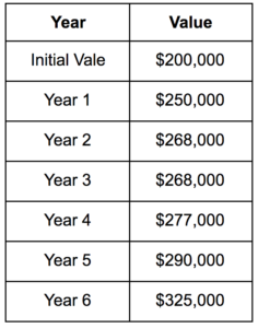
According to this formula, the growth rate for the years can be calculated by dividing the current value by the previous value. For this example, the growth rate for each year will be:
Growth for Year 1 = $250,000 / $200,000 – 1 = 25.00%
Growth for Year 2 = $265,000 / $250,000 – 1 = 6.00%
Growth for Year 3 = $268,000 / $265,000 – 1 = 1.13%
Growth for Year 1 = $277,000 / $268,000 – 1 = 3.36%
Growth for Year 2 = $290,000 / $277,000 – 1 = 4.69%
Growth for Year 3 = $325,000 / $290,000 – 1 = 12.07%
AAGR is calculated by dividing the total growth rate by the number of years.
AAGR = (25% + 6.00% + 1.13%+ 3.36% + 4.69% + 12.07%) / 6 = 8.71%
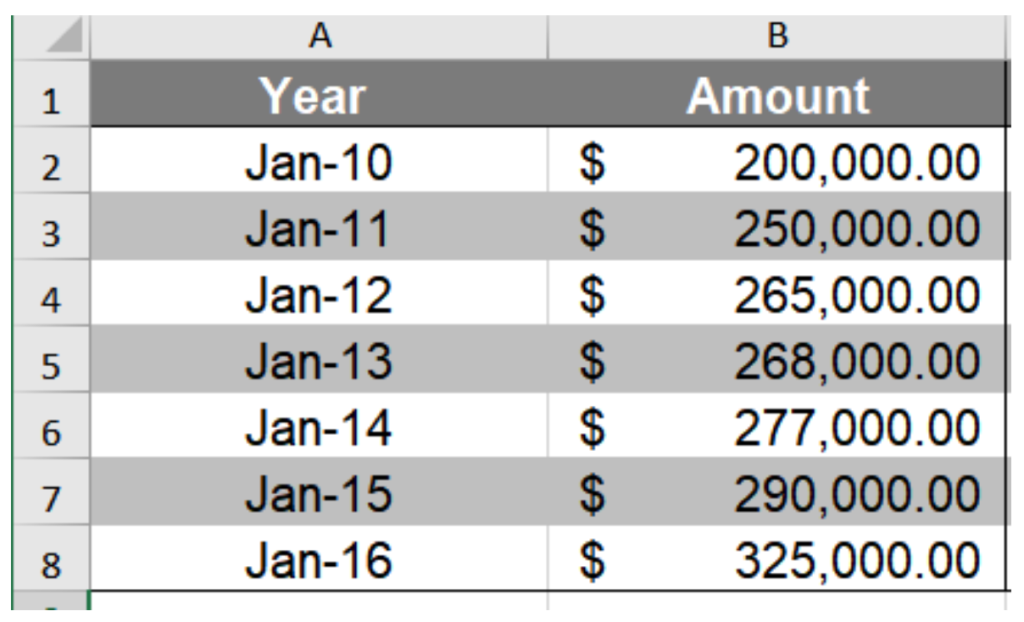
In this example, the cells A1 to B7 contains the data of the example mentioned above.
To calculate AAGR in Excel:
- Select cell C3 by clicking on it by your mouse.
- Enter the formula
=(B3-B2)/B2to cell C3. Press Enter to assign the formula to cell C3.
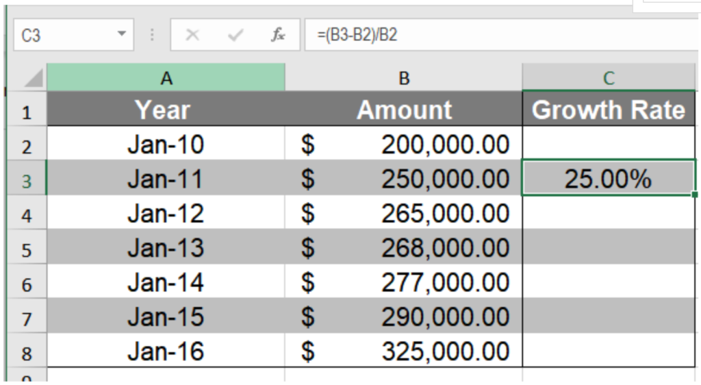
- Drag the fill handle from cell C3 to cell C8 to copy the formula to the cells below.
- Column C will now have the yearly growth rates. Go to cell F4.
- Assign the formula
=AVERAGE(C3:C8). Press Enter.
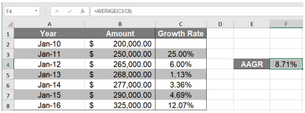
This will show the annual average growth rate of 8.71% in cell F4.
How to calculate the Compound Average Growth Rate
The compound average growth rate is the rate which goes from the initial investment to the ending investment where the investment compounds over time. The equation for CAGR is
CAGR = ( EV / IV)1 / n – 1 where,
EV = Ending Value
IV = Initial Value
n = Time period
For example, if you invest $ 225,000 in a business for five years and the year-end values for every year are:
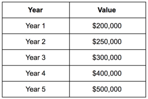
You can calculate CAGR as:
CAGR = (500,000/225,000)1/5-1= .1731=17.32%
Cells A1 to B6 contains the data mentioned above. To calculate CAGR,
- Go to cell E3. Select it with your mouse.
- Assign the formula
=(B6/E2)^(1/(5-1))-1to cell E3. Press Enter to assign the formula to cell E3.
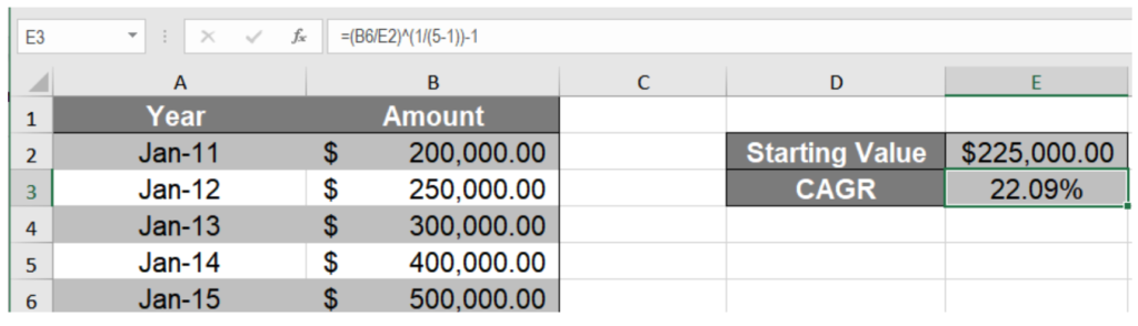
- Cell E3 will have the CAGR value. Format it as a percentage value by clicking on the percentage (%) symbol from Home > Number.
Cell E3 will now show the compound annual growth rate of 22.08%.
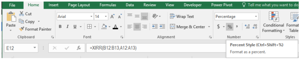
How to calculate the Compound Annual Growth Rate using the XIRR Function
You can also use the XIRR function to calculate CAGR in Excel. The XIRR function in Excel returns the internal rate of return for a series of cash flows which might not occur at a regular interval. The XIRR function uses the syntax =XIRR(value, date, [guess]). It uses the values and their corresponding dates to find the rate of return. You can provide the beginning and end values and corresponding dates as the argument to an XIRR function to find CAGR. To find CAGR from the previous example using the XIRR function:
- Create a new table in cells A11 to B13 with the initial and ending values. Column A has to contain the dates in a Date format in Excel for the XIRR function to work. Make sure to add a minus (-) sign before the ending value. Without this, you will get a #NUM! error.
- Go to cell E12.
- Assign the formula
=XIRR(B12:B13,A12:A13)to cell E12.
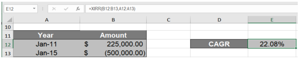
- Press Enter to assign the formula to E12.
Cell E12 will now show the CAGR value 22.09%.
Still need some help with Excel formatting or have other questions about Excel? Connect with a live Excel expert here for some 1 on 1 help. Your first session is always free.
Are you still looking for help with the VLOOKUP function? View our comprehensive round-up of VLOOKUP function tutorials here.


HI, I have an issue
How to troubleshoot crashing and not responding issues with Excel?