Highlight rows with blank cells

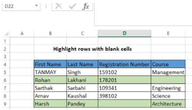
With the help of conditional formatting and a formula based on the COUNTBLANK function, we can easily highlight those rows that have one or more blank cells. This post will provide a clear guide on how to highlight rows with blank cells in excel.

Figure 1: how to highlight rows with blank cells

Syntax of the formula

=COUNTBLANK($B5:$E5)

Understanding the formula

The Excel COUNTBLANK function is fundamental when it comes to highlighting rows that have empty cells. Together with this formula, we will need to understand how to correctly apply conditional formatting so that the rows are highlighted in your preferred color.

It is important to understand that the conditional formatting is entered relative to the active cell in the specified range.

How the formula works

• Conditional formatting is applied relative to the active selection as at the time of entering the rule.
• To prevent columns from changing when the formula is being evaluated, the columns are locked.
• Row references are free to change given that they are relative.
• This formula applies same logic to all the cells in one given row at a time.
• The COUNTBLANK function will return a positive number when it comes across an empty cell. This will trigger the rule and the conditional formatting shall be applied.
• In the event that no empty cell is detected, the function will return a zero, which does not trigger the rule.

Example

Figure 2: Example of how to highlight rows with empty cells

In this example, we want to highlight those rows that have empty cells in them. To do this, we proceed as follows:

Step 1: Fill the excel sheet with data, leaving some cells empty

Step 2: Apply conditional formatting by selecting the range and clicking on the “Conditional formatting” key.

Step 3: Enter the formula; =COUNTBLANK($B5:$F5), then format, specifying the colors you want.

Step 4: Click “Apply” followed by “Ok” to apply the formatting rule.

Instant Connection to an Expert through our Excelchat Service

Most of the time, the problem you will need to solve will be more complex than a simple application of a formula or function. If you want to save hours of research and frustration, try our live Excelchat service! Our Excel Experts are available 24/7 to answer any Excel question you may have. We guarantee a connection within 30 seconds and a customized solution within 20 minutes.

Are you still looking for help with Conditional Formatting? View our comprehensive round-up of Conditional Formatting tutorials here.