

Combine conditional formatting with an IF statement
Syntax
=IF (logical_test, [value_if_true], [value_if_false])
But in conditional formatting, IF/THEN/ELSE syntax cannot be applied in a single rule. Conditional formatting is applied using IF/THEN logical test only. It must return TRUE for conditional formatting to be applied.
For example, if you want to apply conditional formatting using a condition that “If a cell value is greater than a set value, say 100, then format the cell as RED, else format the cell as GREEN”. So, you can see that it requires two rules to perform the conditional formatting, one for greater than 100, and one for less than 100.
You can apply more than one condition by creating more than one rule in conditional formatting. You can also use logical functions like AND and OR to create a rule set and apply conditional formatting in Excel.
Examples using conditional formatting with IF/THEN conditions
Let’s look at the scenarios to see how to use IF/THEN logical test in conditional formatting to highlight the targeted values. If you want to highlight the invoices in data range of A2:C13 which are due in the month of April, then you need to test the IF/THEN logical condition on date range in column B, if the month is equal to April, by using following custom formula in conditional formatting.=MONTH($B2)=4
First, select the data range A2:C13, then go to:
Conditional Formatting (on the Home tab) > New Rule> Use a formula to determine…> Enter the above formula in Edit Rule Description window> Choose the Format Fill to preview and press OK
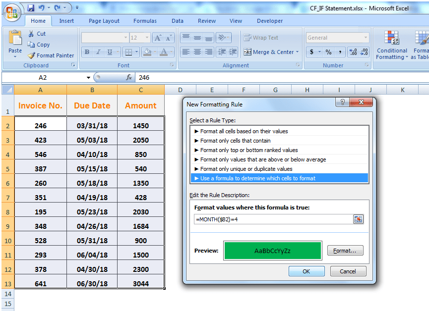
Please note that you have to fix the column by making it absolute using $ sign with it, and keep the row number free or relative to change. Hence, the formula will check each row of the specified column in the selected range, test the IF/THEN logical condition and will return TRUE and FALSE.
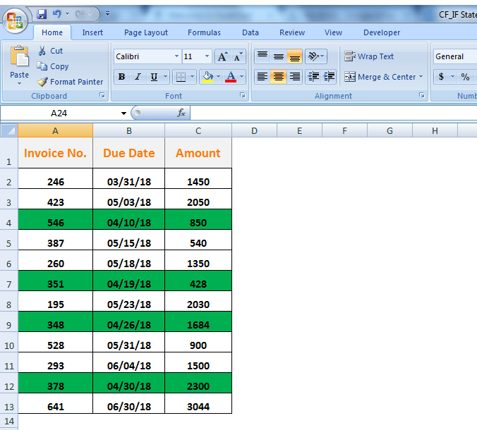
This rule will be evaluated in all active cells of locked column B one by one ignoring other cells in columns A and C. When the MONTH function in a cell of column B returns number 4 (April), the rule will return TRUE for all the active cells in that row and conditional formatting will be applied to that entire row as shown below.
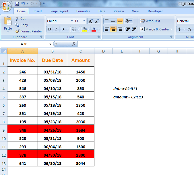
Now, if you want to conditionally highlight the two largest amount invoices due in the month of April, then you can achieve this by creating a rule set based on array formula using AND, LARGE and IF statement as per the following syntax.
=AND(criteria,$C2>=LARGE (IF(criteria, values),2)) =AND(MONTH($B2)=criteria,$C2>=LARGE (IF(MONTH(date)=criteria, amount),2)) =AND(MONTH($B2)=4,$C2>=LARGE(IF(MONTH($B$2:$B$13)=4,$C$2:$C$13),2))
By applying this custom formula, you can highlight the two largest amount invoices in the month of April. LARGE with IF function will generate a series of values and compare them with each value in column C. AND function will test the logical conditions in each cell of column B and C both one by one and will return TRUE where both conditions will be met. Have a look below.
Need some additional help with Conditional Formatting or have other questions about Excel? Connect with a live Excel expert here for some 1 on 1 help. Your first session is always free.


Hi there Im trying to apply conditional formatting to cells that do not contain a formula. I am using excel 2010 so Ive used a macro to create the =ISFORMULA function but the conditional formatting is not working if the formula returns FALSE
I am using duplicate control in excel through Conditional Formatting, total 18,500 nos. of Rows are existing in the sheet. Filter with Highlight Color is not working now. Please suggest me the best way to check duplicacy..
I want to copy Conditional formatting rules, but also the change the rule it applies to based on the cell it is in.
Trying to use conditional formatting to color code cells that are greater or less than another cell. However there is text in the cells and the conditional formatting isn’t correctly color coding values that are higher or lower. Any ideas?
I have a formula of color changing (conditional formatting), just need someone to help fix it!
I want to be able to use conditional formatting to highlight a column of different values in comparison to another column, but all the values vary. I know how to use conditional formatting to highlight a value over or under a set amount but not a varied one?
How to Use Conditional Formatting to Change Cell Background Color Based on Cell Value not for only 1 cell but all the cells depending upon the cell value entered. for example I have four status as 1 )open 2) Resolved 3) Overdue 4) hold. I want the cell should change color as green if resolved and red as overdue and open as brown and hold as yellow.
Hi, I’d like to create format table for work due date 7 days before allot required(like conditional formatting) with different scenarios of production stages. Kindly please help me
I am struggling to create a conditional formatting formula that is dependent on the contents of another cell. which changes color depending on the proximity of the contents of the second cell
I have an issue with my pivot table. I am trying to set the conditional formatting on my pivot. The data in my pivot will change daily. I would like my rule to apply to my data as it adjusts daily. I set my rules but when I filter or make any changes to the data my conditional formatting rule is taken off. How can I get this conditional formatting to stay in place?
I need help with conditional formatting, I cannot seem to make the rules work and apply to the whole sheet.