

The SUMIFS function in Excel sums data that fulfills multiple criteria. It is one of the most widely used math and trig functions to add data based on multiple conditions. In this tutorial, you will learn how to use SUMIFS in Excel.
The SUMIFS Function in EXCEL
Syntax of the Function
SUMIFS(sum_range, criteria_range_1, criteria_1, [criteria_range2, criteria_2], ...)
Arguments within the function
sum_range
Required. The range of cells to sum.
criteria_range_1
Required. The first set of range to be checked.
criteria_1
Required. The value that criteria_range_1 is evaluated against. This defines the cells that will be summed. This can be any number, cell reference, logical expression, text, or another function.
[criteria_range_2, criteria_2,…]
Optional. Additional ranges and their criteria to evaluate. You can add up to 127 range-condition pairs.
Notes About SUMIFS
- The functions SUMIF and SUMIFS have a lot in common. But SUMIFS can evaluate multiple conditions which is not possible for SUMIF. The first argument for SUMIFS is sum_range, whereas it is the third argument for SUMIF.
- All other ranges must have the same number of rows and columns as the sum_range.
- You can use the wildcard characters question mark (?) and asterisk (*) as criteria. A question mark (?) matches one character and an asterisk (*) matches a sequence of characters.
- You must enclose non-numeric criteria in double quotes (“”). i.e., “>144”. But numeric criteria does not require quotes.
- To match a question mark (?) or asterisk (*) in a text, use a tilde (~) in front of the question mark or asterisk. i.e., ~?
- You cannot use SUMIFS with arrays. For this reason, you cannot use functions associated with arrays on the criteria range. For example, you cannot use the YEAR function on criteria_range_1 as it will turn the range into an array. To skip this obstacle, use the SUMPRODUCT function instead.
Examples of the SUMIFS Function
In the following example, you have the sales data for different drinks in three states during a sales campaign.
How to Use SUMIFS in Excel Using Cell References
You can provide cell references as arguments of the SUMIFS function. To find the revenue from the sales of Pina Colada in Alabama (AL):
- Go to cell F6 and click on it.
- Assign the formula
=SUMIFS(C2:C16,A2:A16,F4,B2:B16,F5)to cell F6. - Press Enter to apply this formula to cell F6.
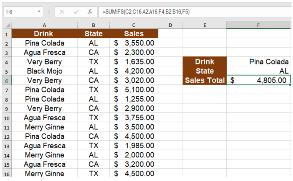
This will show the result $ 4,805, the sum of the sales of Pina Colada in the state of AL during the campaign.
How to use SUMIFS in Excel with Comparison Operators
You can use comparison operators as the arguments of a SUMIFS function to compare with any data type. Make sure to enclose the condition containing the operator in double quotes. To find the sum of sales in AL over $3,000:
- Go to cell F6 and click on it.
- Assign the formula
=SUMIFS(C2:C16,B2:B16,"AL",C2:C16,">3000")to cell F6. - Press Enter to apply this formula to cell F6.
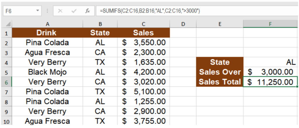
This will show the result $ 11,250, the sum of the sales in the state of AL over $3,000.
Use SUMIFS with Wildcards
You can use SUMIFS with wildcards characters to find similar but not exact matches. You can use the question mark (?) or asterisk (*) character to find matches.

The formula =SUMIFS(C2:C16,A2:A16,"Mer*",B2:B16,"T?") in cell F6 returns the result $ 4,500. Here, the “Mer*” matches the text Merry Ginne and the “T?” matches with the state TX returning the sum of the sales of Merry Ginne in Tx.
Using SUMIF with Blanks
You can use SUMIF with blank cells using the empty string (“”) provided as a criterion to the SUMIF function. In the following example, we have the previous data with the states being cleared out. To find the total sales for Pina Colada:
- Go to cell F6.
- Assign the formula
=SUMIFS(C2:C16,A2:A16,F4,B2:B16,"")to cell F6. - Press Enter.
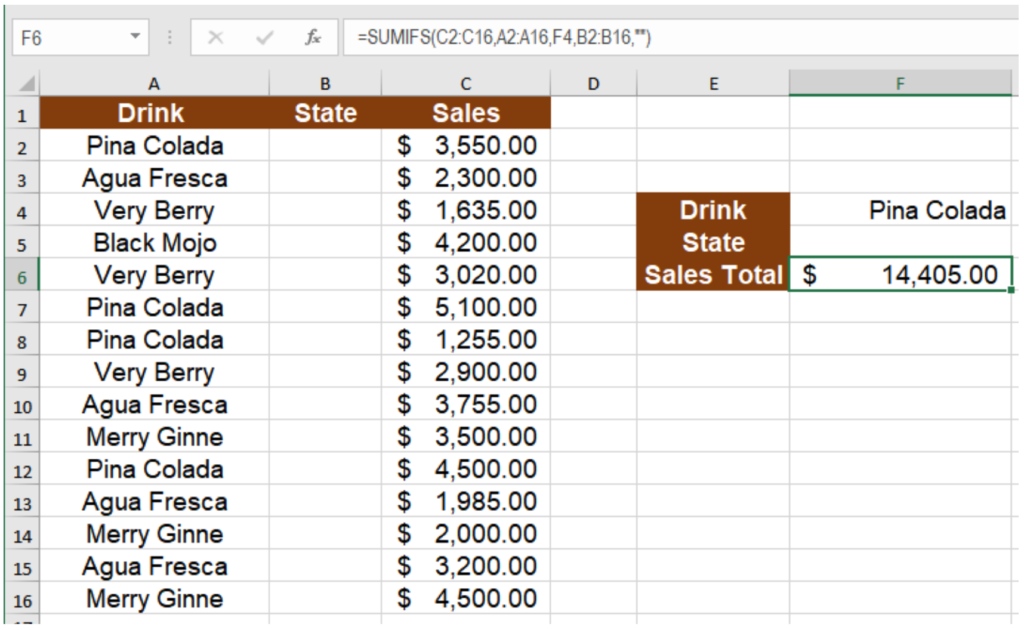
This will return the value $ 14,405 which is the total for the sales of Pina colada. Here the empty string provided as the criterion for the cells B2 to B16 sums the sale for the drinks in A2 to A16 associated with the blank cells in column B.
How to use SUMIFS with Dates
You can use the SUMIFS formula in Excel with dates like any other data types. To sum values between two dates, you can use the ampersand (&) operator along with date functions. The following example contains the employee working hours for the last week. To count the total working hour in the past two days:
- Select cell E6.
- Assign the formula
=SUMIFS(C2:C16,B2:B16,"IT",A2:A16,">="&TODAY()-2,A2:A16, "<="&TODAY())to cell E6. - Press Enter to assign the formula to cell E6.
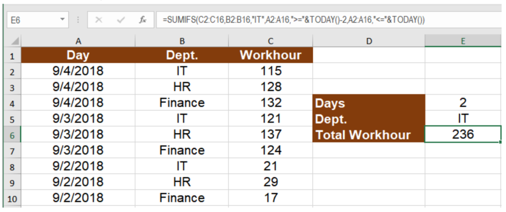
This will show the total work hour 236 for the dept IT in the last two days.
Still need some help with Excel formatting or have other questions about Excel? Connect with a live Excel expert here for some 1 on 1 help. Your first session is always free.


Leave a Comment