

Google Sheets is similar to Excel and uses many of the same functions. Assuming you want to sum a range of values and have some criteria to either include or exclude, you can use the SUMIFS function.
How to Use SUMIFS in Google Sheets
If you want to learn how to use SUMIFS function in Google Sheets, you need to define both sum range from which are values summed and criteria ranges with criterions using the formula: =SUMIFS(sum_range, criteria_range1, criterion1, [criteria_range2, ...], [criterion2, ...]).
The range is defined as the cell range where you want to sum values in Google Sheets and criteria range is the range which we want to filter for certain values, while criterion is the value which we want to take out from criteria range. If you are familiar with this function in Excel, it will be easy for you to use it in Google Sheets.
Some interesting and very useful examples will be covered in this tutorial with the main focus on SUMIFS function; it’s the difference between SUMIF, various ways of usage. After this tutorial, you will be able to sum values based on multiple range criteria or various logical conditions – which is the very good base for further creative Google Sheets problem-solving.
- SUMIFS Function for Multiple Criteria
- SUMIFS with Conditions: Greater Than/Less Than/Equal to/Not Equal to
- SUMIFS Function with OR Criteria
- SUMIFS Function for Multiple Criteria
As we already mentioned above, the main difference between SUMIF and SUMIFS functions is the possibility to define multiple criteria based on which sum is calculated. In this topic, we will explain how the function works with “AND” logical operator when we need all criteria to be met.
A formula using SUMIFS
The formula for SUMIFS function looks like:
=SUMIFS(sum_range, criteria_range1, criterion1, [criteria_range2, ...], [criterion2, ...])
Notice that we can add as much criteria ranges as we need. Let’s look at the example and explain functions parameters:
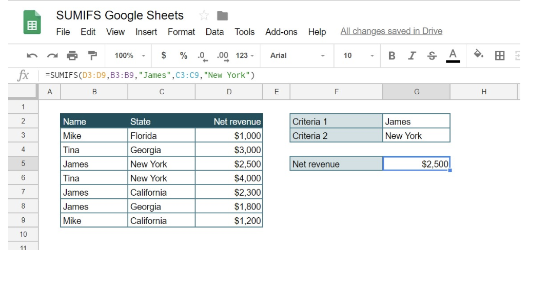
=SUMIFS(D3:D9,B3:B9,"James",C3:C9,"New York")
Explanation of the formula
Sum_range is a range of cells that we want to sum – in our example that would be range A3:A9 (“Net revenue” column). Criteria_range1 is a range which we want to filter for certain values, in our example B3:B9 (“Name” column). Criterion1 is the value which we want to take out from Criteria_range1, in our example “James.” Similarly, Criteria_range2 (C3:C9 – “State” column) and Criterion2 (“New York”) are defined. In other words, we want to sum all Net revenue that has value “James” in “Name” column and “New York” in “State” column.
The previous example consists of passing the certain parameter value to the function (like “James” or “New York”). However, if we want our function to be more dynamic, we can pass cells address to Criterion values, instead of values. In this case, our function would look like:
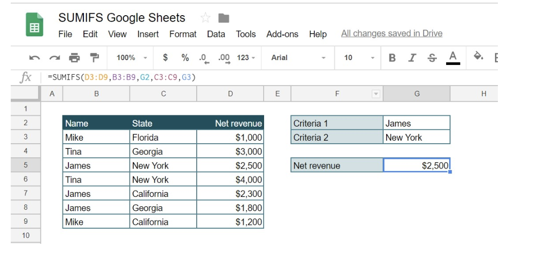
=SUMIFS(D3:D9,B3:B9,G2,C3:C9,G3)
Doing like this, we can change the values of Criteria 1 and Criteria 2 in cells G2 and G3, and our function will be changed accordingly.
SUMIFS with Conditions: Greater Than/Less Than/Equal to/Not Equal to
While working with SUMIFS function, there is often a need to use criteria on value fields or dates. With this data types we usually don’t want to filter just one value, but some range of values like: greater than, less than, between, equal to or not equal to.
In the following example, we will see how to include values comparison in SUMIFS function. Let’s say that we want to keep all criteria from the previous example (Name is Mike and State is New York), but also want to sum only those Net revenues that have the value greater than $1,000:
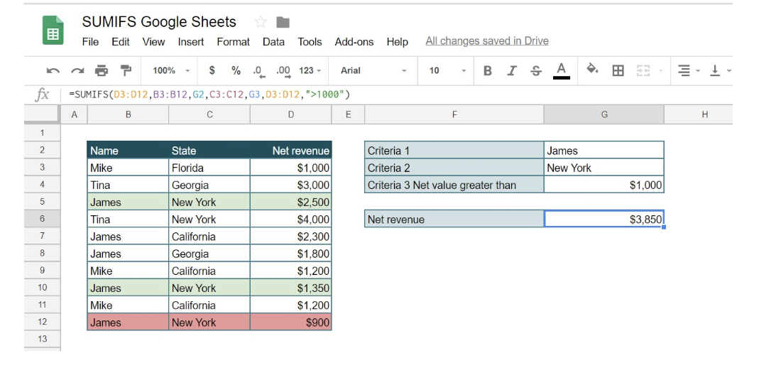
=SUMIFS(D3:D12,B3:B12,G2,C3:C12,G3,D3:D12,">1000")
As you can see, we used the existing function and criteria for Name and State values and added third criteria range D3:D12 (“Net revenue” column). This time for criterion, we put “>1000”, which means that we want to sum up only values greater than $1000. Therefore only rows colored in green were included in sum, while the red row was not, because of the value $900.
Again, we can do this dynamically also:
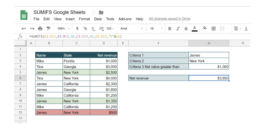
=SUMIFS(D3:D12,B3:B12,G2,C3:C12,G3,D3:D12,">"&G4)
In this case, the criterion is passed to function by putting logical operation (>) in quotations and concatenating it with an ampersand: “>”&G4.
The same logic is used for the following conditions, just with different operator: less than <, greater than or equal to >=, less than or equal to <=.
Additional explanation in this topic is needed for summing values with criteria containing empty or non-blank cells. Let’s first look at the example where we want for one criterion to be always filled (non-blank cells):
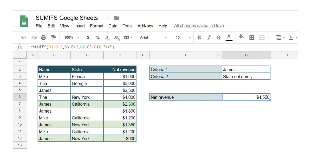
=SUMIFS(D3:D12,B3:B12,G2,C3:C12,"<>")
In this case, we want column “Name” to have value James and for column “State” the only condition is not to be empty. As you can see we get the sum of all Net revenues for James from all States. For criterion “State” we put “<>” which means that we want non-blank cells.
On the other side, let’s look at the example where we want one of our criterion to be empty cell:
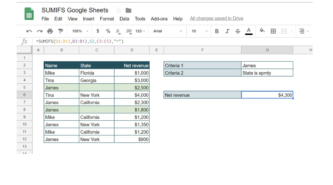
=SUMIFS(D3:D12,B3:B12,G2,C3:C12,"=")
Again, we want column “Name” to have value James, but for column “State” we want to take only empty values. This time we get the sum of all Net revenues for James from State which has no filled cells. For criterion “State,” we put “=” which means that we want only blank cells.
SUMIFS Function with OR Criteria
If we use the SUMIFS function, each criterion in the formula has to be fulfilled in order to calculate formula result correctly. If even one criterion is not met, formula result will be zero, since this function follows AND logic. Question is how to summarize data based on multiple criteria, where either one condition has been met.
Let’s look in the example below where we want to show total Mike Net revenue in Florida or California. This can be done easily by summing two SUMIFS functions, wherein the first part conditions would be “Mike” and “Florida”, and in the second SUMIFS function conditions would be “Mike” and “California”.
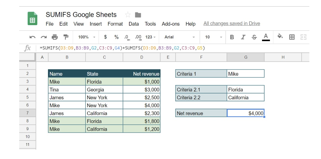
=SUMIFS(D3:D9,B3:B9,G2,C3:C9,G4)+SUMIFS(D3:D9,B3:B9,G2,C3:C9,G5)
Logic is simple. At first, we calculate Net revenue that meets the first part of the condition (Mike, Florida), and then just add separately calculated Net revenue that meets second part of the condition (Mike, California). Instead of writing conditions as text under quotations, it’s always a better solution to link conditions to the cells in order to make reports more dynamic and suitable for changes.
Instead of using SUMIFS function, a more elegant solution is the combination of functions: SUMPRODUCT, ISNUMBER, and MATCH. Take a look in the example below, where the wanted output is James Net revenue in New York or California. Since formula syntax may be looking difficult, we will explain it step by step:
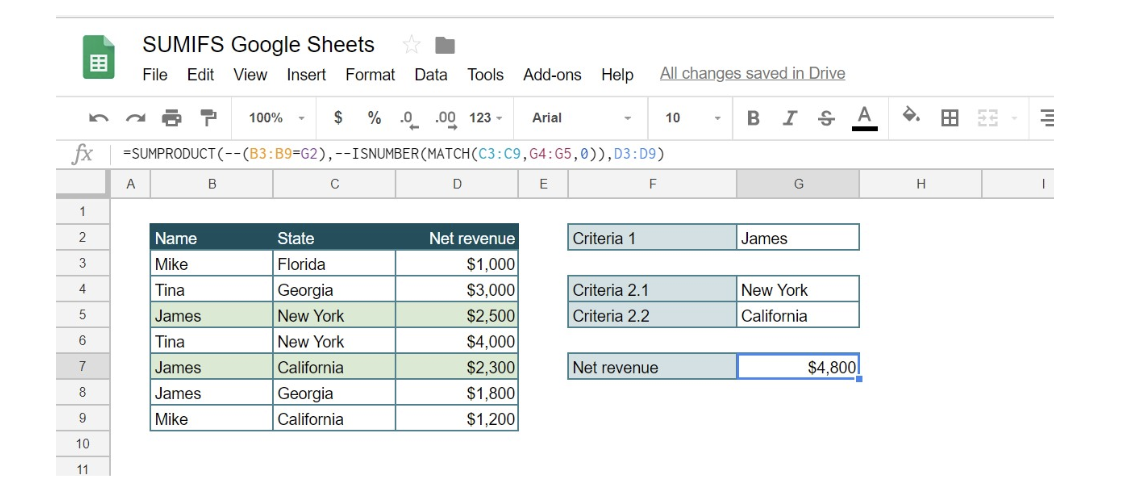
=SUMPRODUCT(--(B3:B9=G2),--ISNUMBER(MATCH(C3:C9,G4:G5,0)),D3:D9)
SUMPRODUCT functions in multiplying arrays in the formula above. The first array is defined with Condition “James”, and whenever the condition is met, formula result is TRUE, and when is not, the result is FALSE. Symbol — in front of the first array (B3:B9=G2) is translating Boolean values TRUE/FALSE into numeric 1/0. Array 1 after formula execution will look like {0,0,1,0,1,1,0}, applying number 1, when condition is met, and 0, when condition is not met in the defined range (Column Name).
In the second array should be checked whether the condition New York or California has been met in Column State. The array should have value 1, whenever New York or California is found in a defined range. This can be done using formula MATCH, with the syntax:
=MATCH(search value,range,0)
Formula MATCH is searching value in a defined range (row/column), and as a result, is giving the position of the searching value in the defined range (row/column). Since we are dealing with arrays, searching value in our example is column State (C3:C9), and range are cells New York and California (G4:G5). Zero in formula syntax is used as we want exact match.
MATCH(C3:C9,G4:G5,0)
After this step array will look like: {#N/A,#N/A,1,1,2,#N/A,2}, showing error when State is not found in range G4:G5, showing 1 if state Now York is found, and value 2 if California is found in range G4:G5. Values 1 and 2, are the positions of searching values in the defined range G4:G5
After this step, formula ISNUMBER is translating array values into Boolean TRUE/FALSE, assigning TRUE if the array value is the number: {FALSE, FALSE, TRUE, TRUE, TRUE, FALSE, TRUE}. Symbol – is then translating Boolean values into 1/0 making array2 looks like: {0,0,1,1,1,0,1}. Now we have a clear array, where number 1 is assigned whenever the condition New York or California is met.
The last array 3 is Net revenue, cell range D3:D9 : {1000,3000,2500,4000,2300,1800,1200}.
At the end, the function is multiplying all three arrays:
{0,0,1,0,1,1,0}*{0,0,1,1,1,0,1}*{1000,3000,2500,4000,2300,1800,1200}=4800
Still need some help with Excel formatting or have other questions about Excel? Connect with a live Excel expert here for some 1 on 1 help. Your first session is always free.


Leave a Comment