How to Use Conditional Formatting to Change Cell Background Color Based on Cell Value

Changing the color of a cell might seem simple enough, but what if you wanted cells to be a particular color based on certain criteria? In these cases, you would use conditional formatting to change your cell’s background color.

Basic cell color formatting

Did you know that you can change the background color of cells by going into the formatting of the cell? Then, you can choose the Fill section and select the intended color to fill the cell.

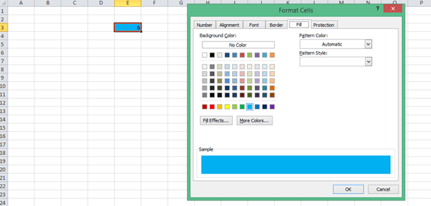
In the above example, the color of cell E3 has been changed from No Fill to Blue color, and notice that the value in cell E3 is 6 and if you change the value in this cell from 6 to any other value the cell color will not change and it will always remain blue.

What does this mean?

This means that cell color is independent of cell value, so no matter what value is entered in E3, the cell color will always be blue. You can refer to this as static formatting of the cell E3.

Cell color formatting based on the cell’s value

Now, what if you want to change the cell color based on cell value? Suppose, you want that color of cell E3 changes with the change of the value in it. Say, you want to color of cell E3 based on values as following.

0 -10: You want the cell color to be Blue

11-20: You want the cell color to be Red

21-30: You want the cell color to be Yellow

Any other value or Blank: No color or No Fill.

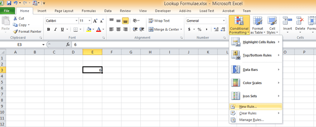
You can achieve this with the help of conditional formatting. On the Home tab, in the style section group, click on Conditional Formatting —–> New Rule

Note: Make sure the cell on which you want to apply conditional formatting is selected.

Then select “Format only cells that contain,” then in the first drop down select “Cell Value” and in the second drop-down select “Between.”

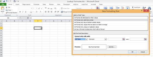
Then, on the first box enter 0 and in the second box enter 10, then click on the Format button and go to Fill Tab, select the blue color, click ok and again click ok.

Now enter the value between 0 and 10 in cell E3, and you will see that cell color changes to blue and if there is any other value or no value then cell color changes to blank.

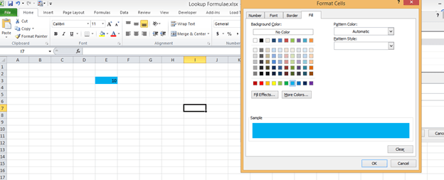
Repeat the same process for 11-20 and 21-30, and you’ll see that number changes as per the value of the cell.

In the example above, you are changing the cell color based on that cell value only. You can also change the cell color based on other cells value as well. Suppose you want to change the color of cell E3 based on the value in D3. To do that, you have to use the formula in conditional formatting.

Now suppose if you want to change the color of cell E3 to blue if the value of cell D3 is greater than 3, and to green, if the value in D3 is greater than 5, and to red if the value is greater than 10.

Again follow the same procedure.

On the Home tab, in the style section group, click on Conditional Formatting —-> New Rule

Note: Make sure the cell on which you want to apply conditional formatting is selected

Now select Use a formula to determine which cells to format, and in the box use the formula, D3>5, then select the formatting to fill the cell color to green.

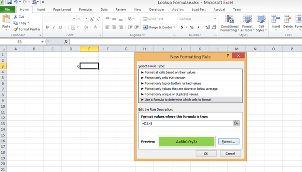
Now notice here that we have selected the cell E3 and not D3, because we want to change the color of cell E3 based on the value of D3. Also, see the formula “=D3>5”, if D3 is greater than 5 then the value of E3 will change to green. Click ok and see the color of cell E3 changes to green as D3 right now contains 6.

Now let’s apply the conditional formatting to E3 if D3 is greater than 3. This means if D3>3 then cell color should become “Blue” and if D3>5 then cell color should remain green as we did it in the previous step.

Now if you follow the above steps as you did for Green color, you will see that even if the cell value is 6, it is still showing blue color and not green. It is because it takes the latest conditional formatting you set for that cell, and as 6 is also greater than 3 hence it is showing blue color, but it should show the green color.

So, you have to arrange the rules you have applied for any particular cells. You can do that by going into the Manage Rules option of conditional formatting.

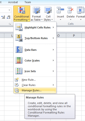
You can see all the rules applied on that cell and there you can arrange the rules or set their priority by using the arrow buttons. A number greater than 5 will also be greater than 3. Hence the rule “greater than 5” will take priority and you have to move it upwards by using the up-arrow button.

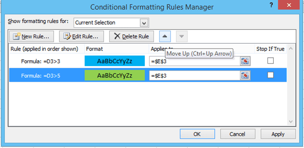
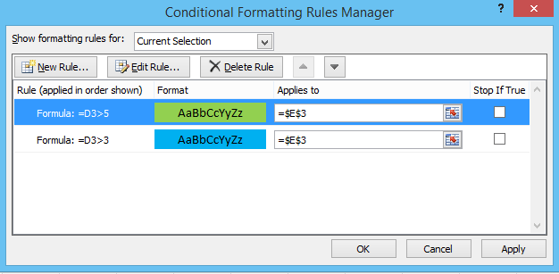
Now when you enter 6 in D3, the cell color of E3 will become green and when you enter 4, the cell color will become blue.

Still need some help with Conditional Formatting or have other questions about Excel? Connect with a live Excel expert here for some 1 on 1 help. Your first session is always free. 

Are you still looking for help with the Average function? View our comprehensive round-up of Average function tutorials here.