

If you want to highlight the entire row of a table based on a value of a specified column as criteria, then you can use Conditional Formatting with a custom formula. When the given condition or criteria meets in the specified column of that table, the formula returns TRUE and resultantly respective row is highlighted with the selected format type.
Highlight a row using conditional formatting in Excel
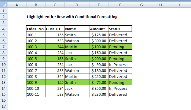
For example, you have a table of customers’ orders and their statuses, let say with a table range of B4:F15 with their respective header names and you want to highlight orders with “Pending” status.
As you can see in below table that column F contains a status of each order. So, column F will be our targeted column where formula will check for given condition to meet.
First, we will select the table range B4:F15, and then we will apply the following formula in conditional formatting to check for a condition:
=$F4="Pending"
Absolute vs. relative cells
Please note that you need to fix the column by making it absolute using $ sign with it, and keep the row number free or relative to change. Hence, the formula will check each row of the specified column in the selected range of table and return TRUE and FALSE.
When you use a formula to apply conditional formatting, the formula is evaluated only in a selected range of cells, also called active cells, with respect to a condition or rule created in the formula. Here, a range of cells B4:F15 are active cells and formula is evaluated in all these cells with respect to rule created above.
As we have locked the column F and kept the row free in the created rule, so this rule will be evaluated in all active cells of locked column F one by one, and other cells in columns B, C, D, and E will be ignored. When the value in a cell of column F is “Pending” the rule will return TRUE for all the active cells in that row and conditional formatting will be applied to that entire row.
You can use another cell as an “input” cell to supply the criteria in the formula and you can easily manage to edit the rule as per your requirement. For example, input the value “Pending” in a cell H4 and use the cell H4 as a reference to provide criteria in the formula above, like:
=$F4=$H$4
Finally, you will select the Format type to preview, like Fill, Font or Border, and apply to take effect. Here we have selected format type Fill > Light Green color to highlight entire row with Light Green background where the condition of status “Pending” meets and formula returns TRUE.
Still need some help with Conditional Formatting or have other questions about Excel? Connect with a live Excel expert here for some 1 on 1 help. Your first session is always free.


Leave a Comment