

Excel provides conditional formatting features for cells or ranges, using which, rule-based formatting standards can be applied easily. In this article, we will learn how to apply conditional formatting for time values in Excel.
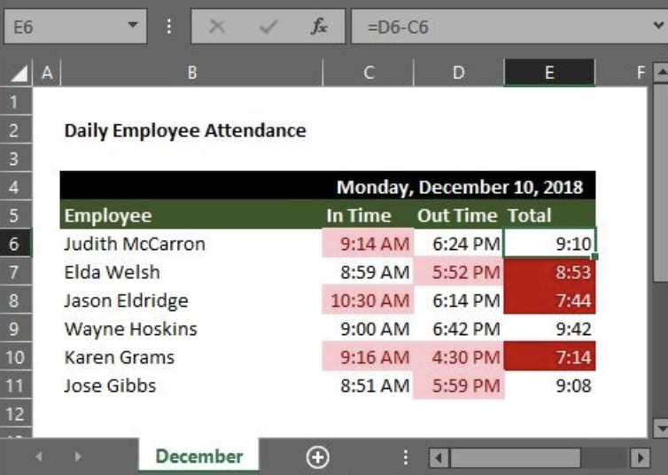
Figure 1. Final result
Steps to apply Conditional Formatting in Excel
Conditional formatting can be applied to individual cells or an entire data range. To apply conditional formatting based on time values, follow the steps below.
- Select the cell or range containing time values
- Click on the Conditional Formatting option found under the Home tab in Excel
 Figure 2. Conditional Formatting feature in Excel
- Select an appropriate formatting rule
Note that Conditional Formatting enables users to highlight cells based on their values. For example, time values that are greater or lesser than a defined value can be highlighted in red.
- Apply the desired formatting
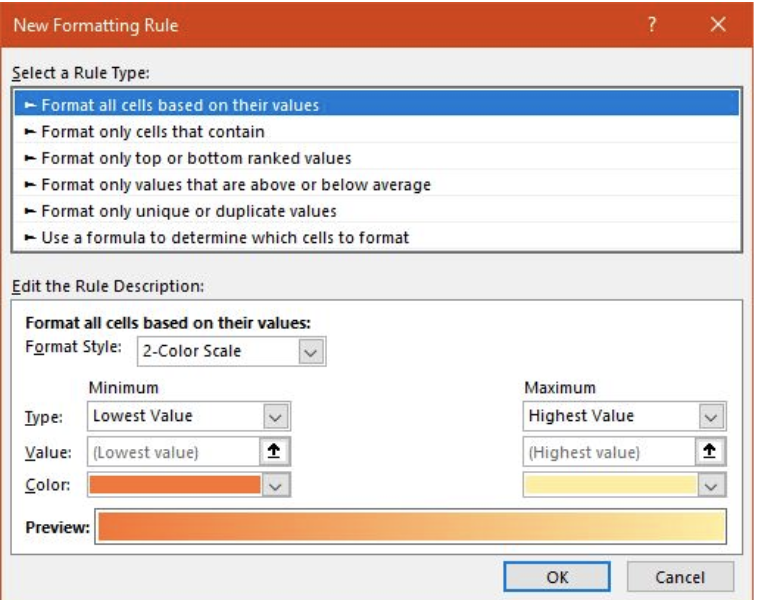 Figure 3. Formatting rules and standards
Example: Employee attendance
Let’s take the example of an attendance log for employees at a company. The basic dataset contains a list of employees with their starting and leaving times, along with a time interval representing total time worked.
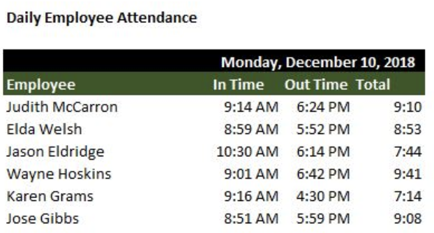 Figure 4. Employee attendance records
Now, we will apply conditional formatting to each column to highlight employees that came to work late (after 9 AM) or left work earlier than their shift ended (before 6 PM). We will apply the following conditional formatting to the first column.
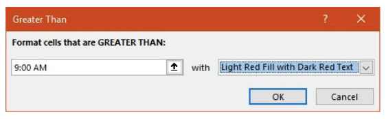 Figure 5. Conditional formatting for employees that came to work late
Similarly, we will apply a “LESS THAN” rule for the Out times, and set the comparator value to 6:00 PM. Here is the end result:
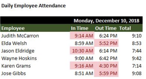 Figure 6. Conditional formatting applied to In and Out times
It is now much easier to identify at a quick glance, which employees came later and/or left the workplace early. We can take this a step further, and apply a custom formatting to the third column, where we will compare time interval value to be less than 9:00 (9 hours). This time, a darker red fill will be used.
Figure 7. Custom formatting applied
Notes
- Excel automatically recognizes values such as “9:14 AM” as valid time values. Two-time values can be simply subtracted to get a time interval
- Conditional formatting can also be applied to time intervals or times that fall within a certain range
- Time-based rules don’t necessarily have to be hard-coded into conditional formatting options. You can use a reference to a cell containing a time value, rather than providing a value directly to the formatter


Leave a Comment