If you need to multiply some corresponding components in a given array and desire to return the sum of the resulting products, then follow these quick basic steps using the SUMPRODUCT function in Excel.
Excel SUMPRODUCT function
The formula in use here is:
=SUMPRODUCT( array1, [array2], [array3], ... [array_n] )
There are 2 basic steps to arrive at this result, and they are as follows:
Step 1: Prepare your Excel workbook with the array of data to be calculated
Step 2: Apply the formula as desired
Formula for SUMPRODUCT
=SUMPRODUCT( array1, [array2], [array3], ... [array_n] )
Step 1:
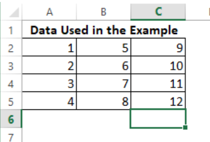
The sample array data is created in the manner as displayed below:
 Figure 1- SUMPRODUCT FUNCTION
Step 2:
At this step, we will go through some series of scenarios where SUMPRODUCT function can be applied to produce results:
SCENARIO 1
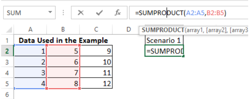
 Figure 2 – SUMPRODUCT FUNCTION
In this first scenario, A2:A5 was used as array1 and B2:B5 was used as array2. The SUMPRODUCT function is calculated on the Cell E2, and the resulting formula is
=SUMPRODUCT(A2:A5, B2:B5)
The above SUMPRODUCT function calculates the selected arrays as =(A2*B2)+(A3*B3)+(A4*B4)+(A5*B5) and results in 70.
SCENARIO 2
 Figure 3- SUMPRODUCT FUNCTION
In this second scenario, A2:B5 is used as array1, and B2:C5 is used as array2. The SUMPRODUCT function is calculated on Cell G2 and the resulting formula is =SUMPRODUCT(A2:B5, B2:C5)
The above SUMPRODUCT function calculates the selected arrays as =((A2*B2)+(A3*B3)+(A4*B4)+(A5*B5))+((B2*C2)+(B3*C3)+(B4*C4)+(B5*C5)) and results in 348.
SCENARIO 3
 Figure 4 – SUMPRODUCT FUNCTION
In this second scenario, A2:A5 is used as array1, and B2:B5 is used as array2. The SUMPRODUCT function is calculated on Cell i2 and the resulting formula is
=SUMPRODUCT(--(A2:A5>2),B2:B5)
This example has a logical function where array1 checks to see data within the array that does not fulfill the logical condition before any calculation is done.
As it happens in all logical conditions, results are returned in the TRUE or FALSE format. The “–” in front of array1 is to change the logical results of TRUE or FALSE to 1 or 0 respectively. This is because the SUMPRODUCT function recognizes only numeric values.
The above SUMPRODUCT function calculates the selected arrays as explained below:
- Since A2 < 2, 0 is reallocated to A2
- Since A3 = 2, 0 is reallocated to A3
- Since A4 > 2, 1 is reallocated to A4
- Since A5 > 2, 1 is reallocated to A5.
Hence this formula is given as:
=(A2*B2)+(A3*B3)+(A4*B4)+(A5*B5)
Which is = (0*5) + (0*6) + (1*7) + (1*8)
The result is 15.
Note
The SUMPRODUCT function can only work with numeric values, and the selection range size of array1 must be same with selection range size of array2 and on till array n.
Still need some help with Excel formatting or have other questions about Excel? Connect with a live Excel expert here for some 1 on 1 help. Your first session is always free.


Leave a Comment