

Changing the cell color based on a value is an effective way to visualize data. Excel has a built-in feature that lets you change the cell color based on value. It’s called Conditional Formatting. Conditional formatting in Excel enables you to highlight cells with a certain color, depending on the cell’s value.
For this tutorial, we will use Naritos food truck annual sales record for the year 2017. Narritos sells Nachos, Burritos, and beverages all over the Bay Area.

Change Cell Color of Top 10 Values
One of the best uses of Conditional Formatting is to quickly highlight top or bottom values in a range. If you do it manually, it would be tedious and take a long time. With conditional formatting, we can do this at once.
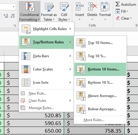
To change the color of top 10 values in a column, at first you need to select the entries in the column, click Home > Conditional Formatting > Top/Bottom Rules> Top 10 Items.

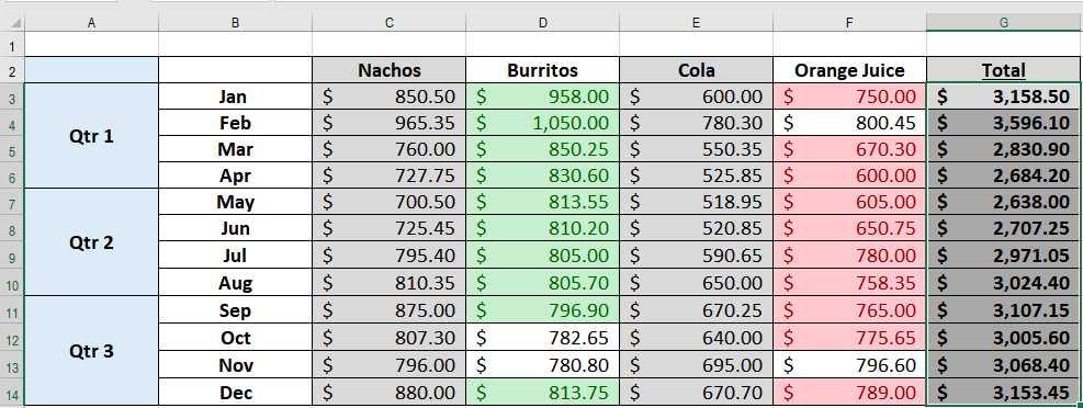
To change the color of the top 10 months that had the highest sale for Burritos, you need to select cells D3:D14, click Home > Conditional Formatting > Top/Bottom Rules> Top 10 Items. Select the fill color as “Green Fill with Dark Green Text” and click OK. This will get an output that looks like this:

Change Cell Color of Bottom 10 Values
You can change the color of the bottom values as well. This can be done following the same process as the top values. After selecting the cells you need to click Home > Conditional Formatting > Top/Bottom Rules> Bottom 10 Items.
To change the color of the bottom 10 months that had the lowest sale for Orange Juice, you’d need to select cells F3:F14, click Home > Conditional Formatting > Top/Bottom Rules> Bottom 10 Items. Select the fill color as “Light Red Fill with Dark Red Text” and click OK. This will get an output that looks like this:
Change Cell Color of Top/Bottom n Values
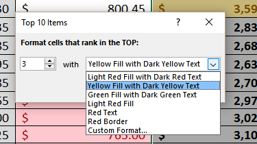
You can change the color of any number top/bottom values with Conditional Formatting. In order to do this, you need to follow similar steps like before. Click Home > Conditional Formatting > Top/Bottom Rules> Top 10 Items. Now set the n value on the window that appears. This will change the color of the top n values in a column. You can change the color of the bottom n values following the same process. In that case, you would need to select the bottom 10 items and follow the previous steps.
To color the top 3 months with the highest sales, you need to select cells G3:G14, Home > Conditional Formatting > Top/Bottom Rules> Top 10 Items. Set the N value to 3 on the left and select the format to “Yellow Fill with Dark Yellow Text” and click OK. This will highlight the top 3 months with the highest sales, which are January, February, and December.
How to Change Cell Color of Top/Bottom 10 Values of Each Category
You can also change the cell color of top/bottom values of cells when there are multiple categories. Excel comes with many “presets” that make it easy to create new rules. However, you can also add your own formula to create rules based on logic.
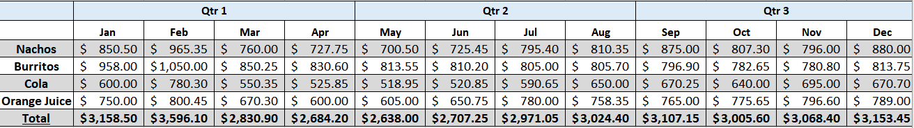
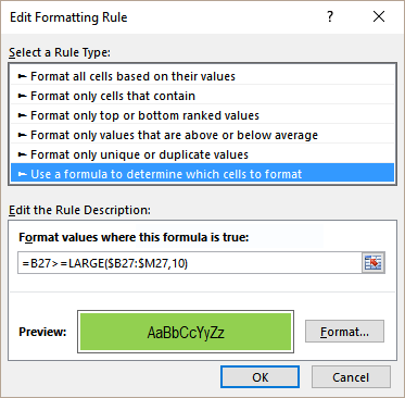
Here we have the Norritos food truck sales data with the items in the rows. To find out the top 10 months for both Nachos and Burritos, you need to select the cells in B27:M28 and click Home > Conditional Formatting > New Rule. Select “Use a formula to determine which cells to format”and on the input window assign the formula,“=B27>=LARGE($B27:$M27,10)” click on Format, set the fill color of your choice. Click OK twice.
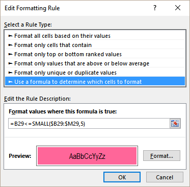
You can change the cell colors of the bottom 5 cells for multiple categories in the same way. To find the bottom 5 values for beverage, you need to select the cells in D29:M30 that has the sales for beverage, Cola and Orange Juice. Now, click Home > Conditional Formatting > New Rule. Select “Use a formula to determine which cells to format” and on the input window assign the formula,“=B29>=SMALL($B29:$M29,5)” click on Format, set the fill color of your choice. Click OK twice.
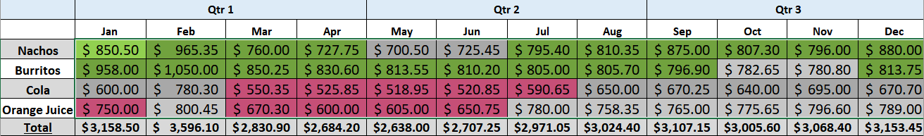
Applying these formats will make the table look like this:
Most of the time, what you need isn’t as straightforward, depending on your situation, there might be other solutions to your problem. If you are in a rush and want your problem answered by an Excel expert, try our ExcelChat help service. The experts are available to help you 24/7 at this link. The first question is free.


Leave a Comment