Conditional formatting based on another cell

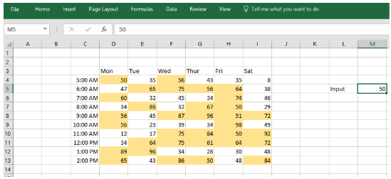
Figure 1. Conditional formatting based on another cell

The general formula

=A1>=$J$1

This formula is used to execute conditional formatting using the value specified in a different cell, a rule can be created using the simple formula. The screenshot above shows the formula employed when using conditional formatting on the array of values between D4 and I13

=D4>=$M$5

How does the formula work?

In Excel, there are so many built-in settings that can be used to highlight cells with conditional formatting. These preset include one used to highlight numbers greater than the specified value. Nevertheless, using a formula give you a lot more control and flexibility.
In the example above, a rule is used to indicate cells between the range of values D4:I13 whenever a number is higher than the specified number in cell M5. The rule is created using this formula:
=D4>=$M$5

Explanation

The entire array of numbers between the range D4 and I13 is tested and the set value in M5 can be easily adjusted. When the value in M5 is adjusted the highlighted values are instantly updated to obey the new condition.
The rule given by the formula adopts the >(“greater than”) or = (“equal to”) operator to test the specified array of numbers against the number entered in cell M5. The formula uses the greater than or equal to operator (>=) to evaluate each cell in the range against the value in M5.
At any instance when a number in the array is higher or equal to the number in cell M5 (50 in the example shown), True is returned. This indicates that the rule has been satisfied.

Are you still looking for help with Conditional Formatting? View our comprehensive round-up of Conditional Formatting tutorials here.