

We often want to enhance the layout and format of our pivot tables by using Conditional Formatting. This step by step tutorial will assist all levels of Excel users in working with a pivot table that has conditional formatting, and learning to solve some common problems associated with it.
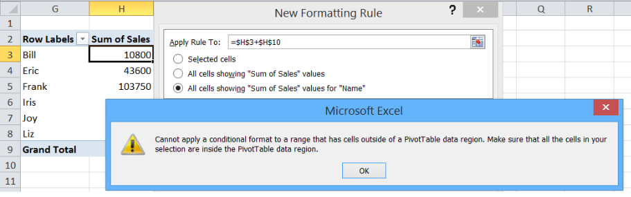 Figure 1. Working with pivot table that has conditional formatting
Setting up Our Data
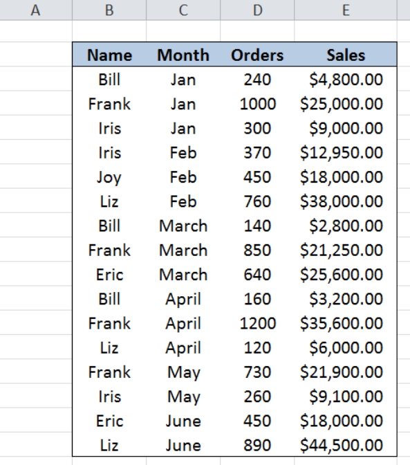 Figure 2. Sample data: Working with pivot table that has conditional formatting
Our table consists of four columns: Name (column B), Month (column C), Orders (column D) and Sales (column E). First, let us insert a pivot table using our data.
Insert a pivot table
In order to insert a pivot table, we follow these steps:
Step 1. Select the cells of the data we want to use for the pivot table. In this case, select cells B2:E18
Step 2. Click the Insert tab, then select PivotTable
 Figure 3. Selecting the data to insert a pivot table
Step 3. In the Create PivotTable dialog box, tick Existing Worksheet. Click the Location bar and then click cell G2.
 Figure 4. Inserting a pivot table in existing worksheet
Step 4. In the PivotTable Field List, click Name, Month and Total Sales
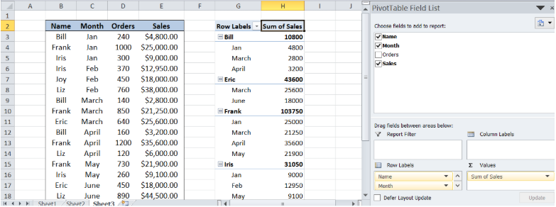 Figure 5. Creating a pivot table with chosen fields
We have now successfully created our pivot table. Now we will discuss three common problems associated with pivot table that has conditional formatting:
- Highlighting the wrong cells
- Conditional formatting not applied to new data added
- Error: Cells outside the PivotTable data region
Highlighting the wrong cells
We want to highlight the sum of sales per month, but the highlighted cells are the subtotals per name as shown below in cells H7 and H10.
 Figure 6. Wrong cells are highlighted through conditional formatting
Work-around
Change the cell reference in the Apply Rule to: bar from $H$3 to $H$4 then tick All cells showing “Sum of Sales” values for “Month”.
 Figure 7. Entering correct formatting range to highlight correctly
This way, the sum of values for each month that are above average are highlighted.
Conditional formatting not applied to new data added
In below table, we have added new data in row 19 for Liz in June. The pivot table has been updated but conditional formatting is not applied to the new data in G24:H24.
 Figure 8. Conditional formatting not applied to newly added data
The most probable cause would be the cell reference or range inside the Apply Rule To: bar.
 Figure 9. Wrong formatting range entered in formatting rule
Work-around
Change the formatting range from $H$3:$H$23 to $H$3:$H$24 to include the newly added data in conditional formatting.
 Figure 10. Entering correct formatting range to include newly added data
Cells outside the PivotTable data region
Sometimes we encounter this error when applying conditional formatting to our pivot table. It says conditional formatting cannot be applied because the range has cells outside of a PivotTable data region.
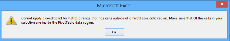 Figure 11. Error in Conditional Formatting: Cells outside PivotTable data region
In cases like this, the Apply Rule To: contains an invalid range like the example below, where the range is: =$H$3+$H$10.
 Figure 12. Invalid formatting range causing error
Work-around:
Make sure that the cell or range in the Apply Rule To: box is inside our pivot table. Let us correct the example and enter the following as range: =$H$3:$H$9
 Figure 13. Entering a valid formatting range
The conditional formatting now works perfectly and highlights the sum of sales above average.
Most of the time, the problem you will need to solve will be more complex than a simple application of a formula or function. If you want to save hours of research and frustration, try our live Excelchat service! Our Excel Experts are available 24/7 to answer any Excel question you may have. We guarantee a connection within 30 seconds and a customized solution within 20 minutes.


Leave a Comment