

While working with Excel, we are able to randomly sort values in a list and display them in a certain order by using the INDEX, MATCH and ROWS functions. This step by step tutorial will assist all levels of Excel users in randomly sorting values using a formula with INDEX, MATCH and ROWS functions.
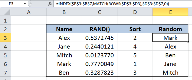 Figure 1. Final result: Random sort formula
Final formula: =INDEX($B$3:$B$7,MATCH(ROWS($D$3:$D3),$D$3:$D$7,0))
Syntax of the INDEX function
INDEX function returns a value from within a range, as specified by the row and column number
=INDEX(array, row_num, column_num)
The parameters are:
- array – a range of cells where we want to retrieve some data
- row_num – the row in the array from which we want to retrieve data
- column_num – the column in the array from which we want to retrieve data; if the array has only one column, column_num can be omitted
Syntax of the MATCH function
MATCH function returns the position of a value in a range
=MATCH(lookup_value, lookup_array, [match_type])
The parameters are:
- lookup_value – a value which we want to find in the lookup_array
- lookup_array – the range of cells containing the value we want to match
- [match_type] – optional; the type of match; if omitted, the default value is 1; We use 0 to find an exact match
Syntax of the ROWS function
ROWS function returns the number of rows in a data set
=ROWS(array)
- array– an array, range or reference for which we want to determine the number of rows
Setting up Our Data
Our table consists of four columns: Name (column B), RAND() (column C), Sort (column D) and Random (column E). In this example, we have two helper columns, column C and column D. Helper columns are columns we set-up to aid us in our computations.
In column C, we enter random numbers given by the RAND() function. As shown below, the formula in cell C3 is =RAND().
 Figure 2. Sample data using RAND function to assign random values
In column D, we rank the values in column B from 1 to 5, with 1 being the highest. The formula in cell D3 that we use for sorting looks like this:
=RANK(C3,$C$3:$C$7)+COUNTIF($C$3:C3,C3)-1
Copying the formula in D3 to cells D4:D7 will give the rank of the values in column B from 1 to 5. The results of ranking will be used in our random sort formula.
![]() Figure 3. Using RANK and COUNTIF to sort random values in column C
Figure 3. Using RANK and COUNTIF to sort random values in column C
Ultimately, what we want to accomplish is to create a list of names in column E, ranking them from 1 to 5 according to the values in column D “Sort”.
Randomly sort names
We want to sort and display the names in column E, considering their ranking from 1 to 5 in column D. Let us follow these steps:
Step 1. Select cell E3
Step 2. Enter the formula: =INDEX($B$3:$B$7,MATCH(ROWS($D$3:$D3),$D$3:$D$7,0))
Step 3: Press ENTER
Step 4: Copy the formula in cell E3 to cells E4:E7 by clicking the “+” icon at the bottom-right corner of cell E3 and dragging it down
The dollar signs “$” in the formula fix the cells so that we can easily copy and paste the formula to other cells.
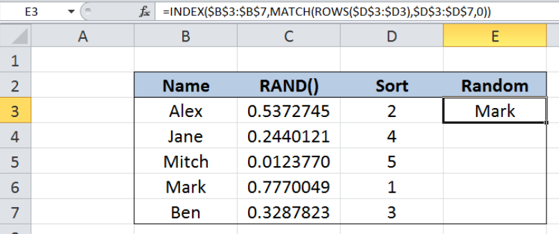 Figure 4. Using INDEX, MATCH and ROWS to find the randomly ranked 1
Our array for the INDEX function is the range B3:B7. Since there is only one column, we can omit the column_num in our formula. The row_num is determined by the MATCH function : MATCH(ROWS($D$3:$D3),$D$3:$D$7,0)
Our lookup_value for the MATCH function is ROWS($D$3:$D3), which returns the number of rows of D3:D3, whose value is 1. Hence, we want to match the value 1 in the lookup_array D3:D7 {2;4;5;1;3}. The value 1 is the fourth value in the array so the MATCH function returns 4.
Finally, the INDEX function returns the fourth row in the range B3:B7, which is B6, or “Mark”. The result displayed in cell E3 is “Mark”, who ranks first as displayed in column D.
For the 2nd to fifth names, the ROWS function provides the ranking we are trying to find, where each new row adds 1 to the result of ROWS. For example in E4, ROWS($D$3:$D4) returns 2, so the MATCH will find 2 in D3:D7 {2;4;5;1;3} and return the value “1”, corresponding to its position in the array.
Below table shows the names in column E that are sorted randomly with the aid of two helper columns.
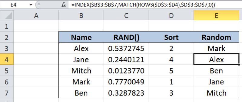 Figure 5. Output: Random sort formula
Most of the time, the problem you will need to solve will be more complex than a simple application of a formula or function. If you want to save hours of research and frustration, try our live Excelchat service! Our Excel Experts are available 24/7 to answer any Excel question you may have. We guarantee a connection within 30 seconds and a customized solution within 20 minutes.


Leave a Comment