

While working with Excel, we are able to determine the number of values that satisfy one or more criteria within a specified range by using the COUNTIFS function. This step by step tutorial will assist all levels of Excel users in generating a course completion summary with criteria.
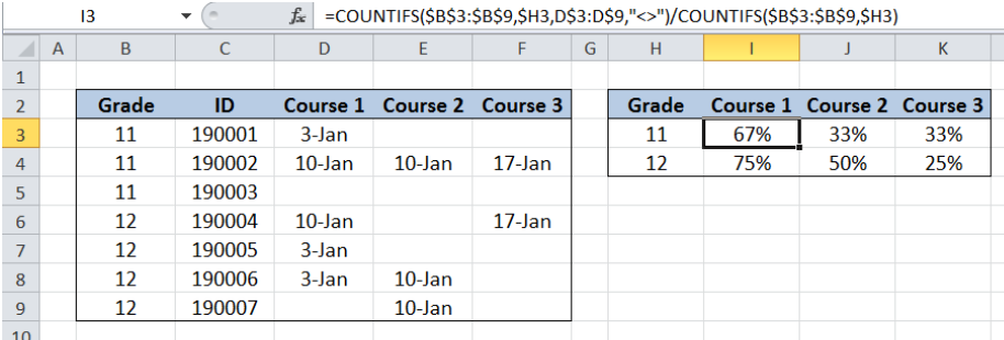 Figure 1. Final result: Course completion summary with criteria
Final formula: =COUNTIFS($B$3:$B$9,$H3,D$3:D$9,"<>")/COUNTIFS($B$3:$B$9,$H3)
Syntax of COUNTIFS Function
=COUNTIFS(criteria_range1, criteria1, [criteria_range2, criteria2]…)
Parameters:
- Criteria_range1: the data range that will be evaluated using the criteria1
- Criteria1: the criteria or condition that determines which cells will be counted
- Criteria_range2 and criteria2 are optional; only applied when there are more than one criteria as specified
Setting up Our Data
Our table consists of five columns: Grade (column B), ID (column C), Course 1 (column D), Course 2 (column E) and Course 3 (column F). Cells H3 and H4 contain our criteria which classifies course completion by grade: Grade 11 and Grade 12.
We want to summarize the completion of each course by grade in percentage form. The resulting percentage of completion per course will be reflected in columns I, J and K.
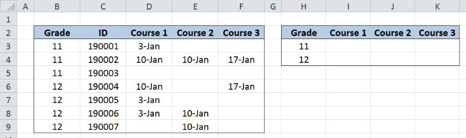 Figure 2. Sample data to summarize course completion with criteria
Course completion summary with criteria
We want to determine the completion of each course with grade as criteria.
Course completion summary for Grade 11
To summarize course completion for Grade 11, we follow these steps:
Step 1. Select cell I3
Step 2. Enter the formula: =COUNTIFS($B$3:$B$9,$H3,D$3:D$9,"<>")/COUNTIFS($B$3:$B$9,$H3)
Step 3: Press ENTER
Step 4: Copy the formula in cell I3 to cells J3 and K3 by clicking the “+” icon at the bottom-right corner of cell I3 and dragging it to the right.
The dollar signs “$” in the formula fix the cells so that we can easily copy and paste the formula to other cells.
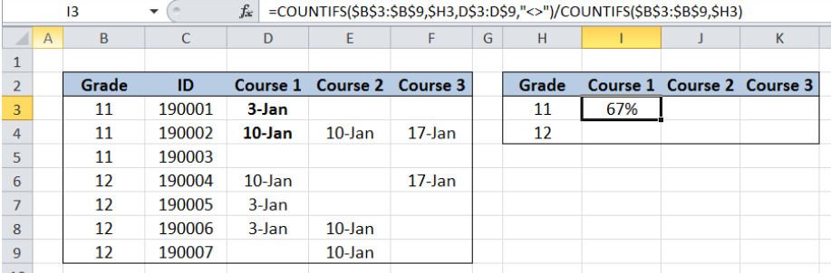 Figure 3. Using COUNTIFS to determine completion of Course 1, Grade 11
Our formula consists of two COUNTIFS functions. The first COUNTIFS determines the count of Grade 11 students who completed Course 1, while the second COUNTIFS determines the total count of Grade 11 students.
The first COUNTIFS has two criteria. It only counts the cells that satisfy both criteria:
- cells in B3:B9 with values equal to H3 or grade “11”
- cells in D3:D9 that are not empty; the symbol “<>” means non-empty text string
The first COUNTIFS returns the value 2, for the two Grade 11 students who completed Course. The second COUNTIFS returns the value 3, for the three Grade 11 students. As a result, the value in cell I3 is ⅔ or 67%.
Below table shows the course completion summary for Grade 11.
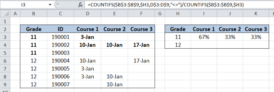 Figure 4. Output: Course completion summary with grade 11 as criteria
Course completion summary for Grade 12
To summarize course completion for Grade 12, we follow these steps:
Step 1. Select cell I4
Step 2. Enter the formula: =COUNTIFS($B$3:$B$9,$H4,D$3:D$9,"<>")/COUNTIFS($B$3:$B$9,$H4)
Step 3: Press ENTER
Step 4: Copy the formula in cell I4 to cells J4 and K4 by clicking the “+” icon at the bottom-right corner of cell I4 and dragging it to the right.
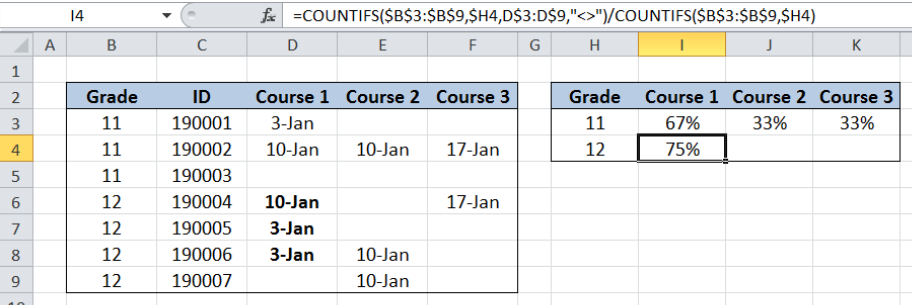 Figure 5. Entering the formula for completion of Course 1, Grade 12
The procedure is the same as in our previous example. Only this time, the criteria used is H4 or grade “12”. Our formula counts the number of Grade 12 students who completed Course 1, which is “3”. It then divides the sum with the total count of Grade 12 students, which is “4”.
The formula returns the value ¾ or 75% in cell I4.
Below table shows the course completion summary for Grade 12.
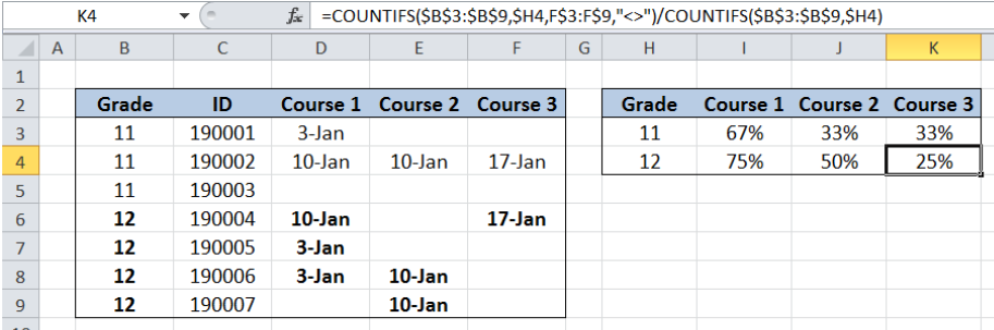 Figure 6. Output: Course completion summary with grade 12 as criteria
Most of the time, the problem you will need to solve will be more complex than a simple application of a formula or function. If you want to save hours of research and frustration, try our live Excelchat service! Our Excel Experts are available 24/7 to answer any Excel question you may have. We guarantee a connection within 30 seconds and a customized solution within 20 minutes.


Leave a Comment