

Conditional Formatting is a built-in feature in Excel, and it enables you to visualize the data by adding some user-friendly formatting based on certain rule types. As you add some basic formatting to your data set to make it more appealing and colorful, like choosing the font size, colors, headers, etc., so when you want to select or apply such formatting types based on some condition, and then it is called Conditional Formatting.
The Conditional Formatting feature in Excel
This feature in Excel enables you to view how a cell appears based on the value of that cell. For example, you may want to highlight a cell with a certain background color, say Red, only if the value in that cell is greater than a certain set value. It is very easy to use conditional formatting because it contains some built-in formatting rules and styles, or you can create your own condition based on your rule or condition type.
Here you are going to use the built-in conditional formatting rules and styles for your data set. After opening your data sheet in Excel and selecting the cells range to apply conditional formatting, on the Home tab, in the Styles group, click on the Conditional Formatting menu.
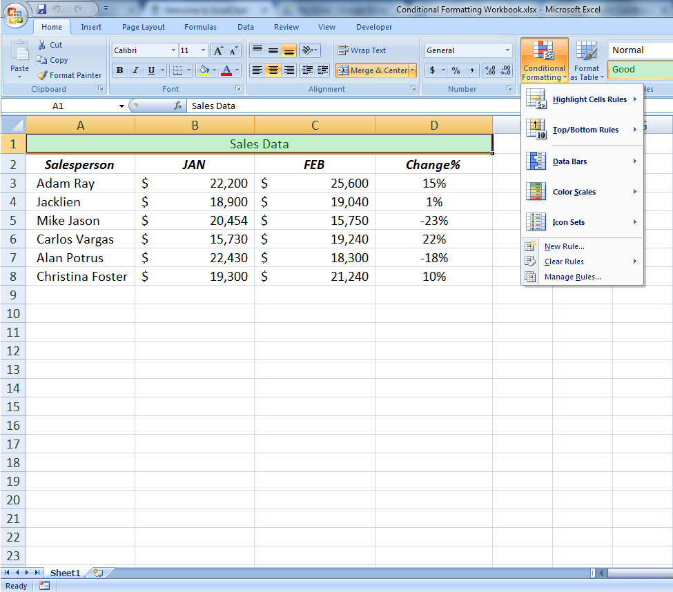
Now you can see the complete list of conditional formatting menu and can choose one of the built-in conditional formatting and styles options to apply to your cells.
Using Built-in Conditional Formatting Rules
Built-in conditional formatting rules section has two menu options to choose from to highlight cells per your requirements.
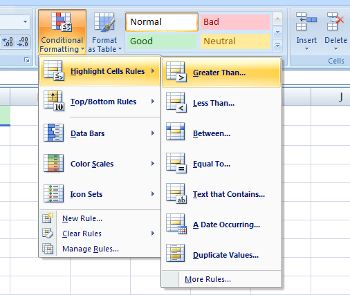
- Highlight Cells Rules. You can conditionally highlight your data range by choosing one of the options from the Highlight Cells Rules menu, or you can create more rules to apply. This menu has some preset conditional formatting rules set and formatting types to apply:
![How to Use Conditional Formatting in Excel]()
You need to choose one of the preset rules and formatting types to apply conditional formatting.
- Greater Than – Highlight cells that are greater than a value you set.
- Less Than – Highlight cells that are less than a value you set.
- Between – Highlight cells that have values between values you set.
- Equal To – Highlight cells that are exactly equal to a value you set.
- Text that Contains – Highlight cells that contain strings of text.
- A Date Occurring – Highlight cells based upon the date in a cell.
- Duplicate Values – Highlight cells which contain duplicate data values.
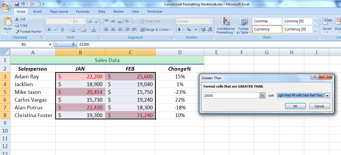
For example, if you want to highlight cells that are greater than a value you set of 20,000 in a selected data range, then you will choose Greater Than rule option and will enter 20,000 in a popup window and will choose a formatting type from the drop-down list as shown below.
![How to Use Conditional Formatting in Excel]()
It will highlight all the cells with “Light Red Fill..” that have value great than your set value of 20,000.
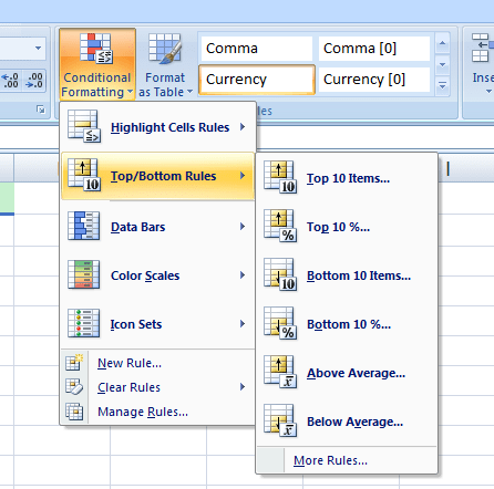
- Top/Bottom Rules. You can easily conditionally highlight your data by choosing one of the Top/Bottom Rules options, or you can create more rules to apply. This menu also has following preset conditional formatting rules set and formatting types.
![How to Use Conditional Formatting in Excel]()
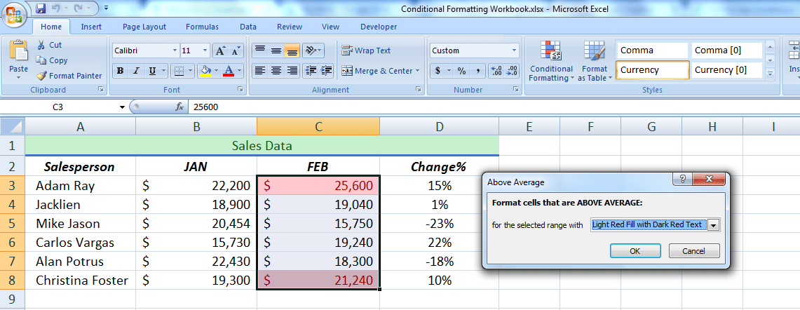
For example, if you want to highlight cells in a particular month in which values are above average, then you will select your data range and choose Above Average option from preset rules and choose to format with an option from popup window as shown below.
It will highlight all those cells with Light Red Fill…. that have values above the average of the selected data range.
![How to Use Conditional Formatting in Excel]()
Using Built-in conditional formatting Styles
If you want to try some more conditional formatting options, then Excel as some built-in styles to use for this purpose, like Data Bars, Color Scales, and Icons Sets.
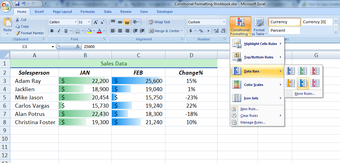
- Data Bars. You can quickly place some colorful Data Bars inside of data cells to represent the size of your data in the selected data range. First, you need to select your data range and then click on the Data Bars menu and choose one of the options to apply as shown below.
![How to Use Conditional Formatting in Excel]()
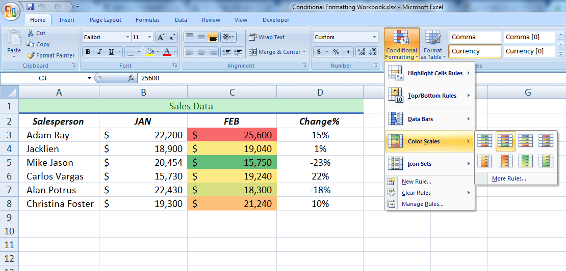
- Color Scales. Color scales highlight the highest and lowest values represented with distinct color patterns in a selected data range. After selecting the data range, you need to choose one of the options from Color Scales menu. The shade of the color represents the value in the cell as shown below.
![How to Use Conditional Formatting in Excel]()
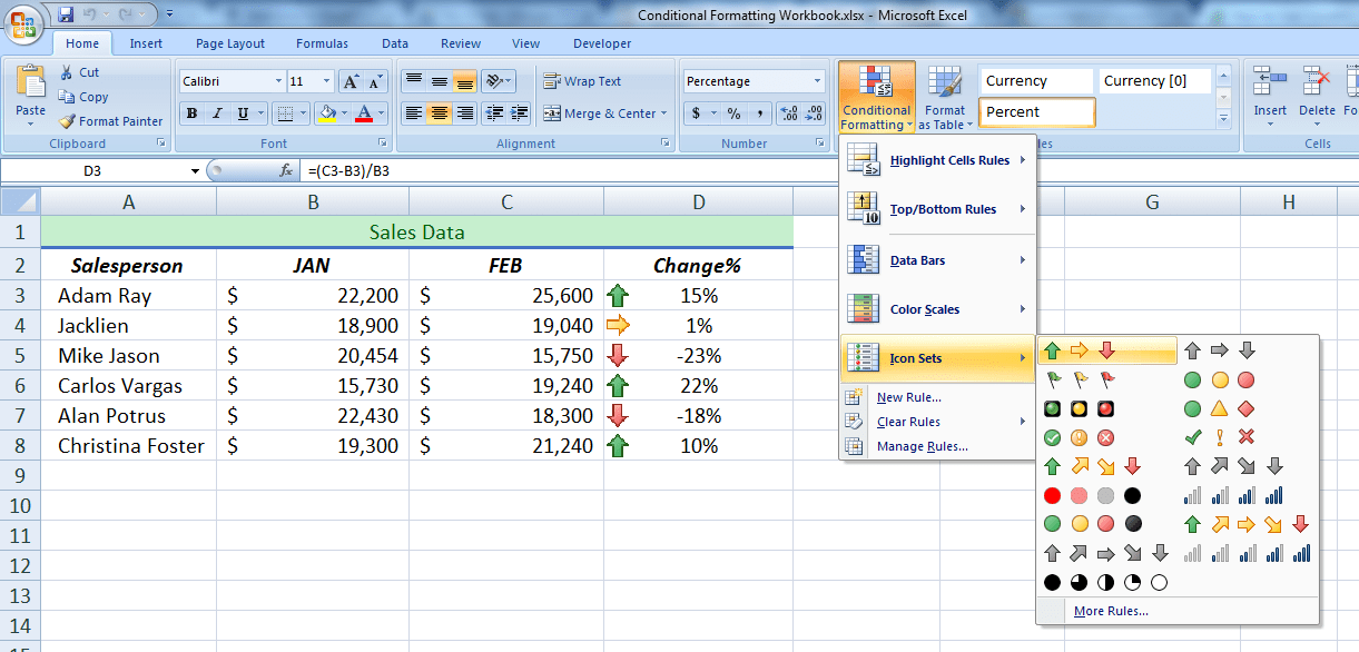
- Icon Sets. The Icon sets show changes in your data. They include arrows, flags, bars, and other shapes to represent the change in your data. Each icon represents a value in the cell as shown below.
![How to Use Conditional Formatting in Excel]()
These Icon sets change when the data changes in the selected range. When the Change% figure changes, Excel will automatically change the icon set accordingly.
If you have trouble using conditional formatting and want to save hours of researching, try our Excel Chat live help service. Our experts are available 24/7 and ready to answer any Excel related question on the spot. The first question is free.


Leave a Comment