

VLOOKUP function is one of the most popular and widely used functions in Microsoft Excel. Learning a few tips would go a long way for us to be able to master the VLOOKUP function. This step by step tutorial will assist all levels of Excel users in learning the best practices for VLOOKUP with table array.
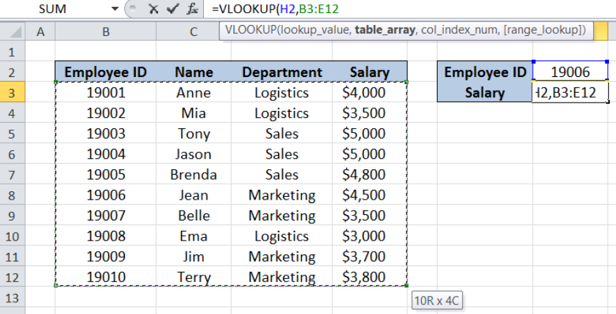 Figure 1. VLOOKUP with table array: 5 best practices
Syntax of VLOOKUP function
=VLOOKUP(lookup_value, table_array, col_index_num, [range_lookup])
The parameters of the VLOOKUP function are:
- lookup_value – the value that we want to search and find in the table_array
- table_array – the range of cells in the source table containing the data we want to retrieve
- col_index_num – the column number in the table_array corresponding to the information we want to retrieve, relative to the lookup_value
- [range_lookup] – optional; value is either TRUE or FALSE
- if TRUE or omitted, VLOOKUP returns either an exact or approximate match
- if FALSE, VLOOKUP will only find an exact match
5 Best Practices
In this article we will learn five best practices that will help us master VLOOKUP and maybe make us a pro one day. VLOOKUP is a complicated function and using the following tips and best practices will tremendously help us:
- VLOOKUP counts column numbers
- Absolute references lock cells in place
- Use IFERROR to trap errors and display a customized result
- VLOOKUP easy to read and maintain using range names
- Use VLOOKUP to categorize data
Excel VLOOKUP counts column numbers
The column index number can be hard to determine especially when we are dealing with a large data set. Column index number is determined by counting columns to the right of the lookup value.
TIP: When we highlight our table array, Excel displays the row and column numbers of the cell we have selected, relative to the first cell. As shown in the table below, we are about to enter the table array B3:E12.
Notice the value at the lower right corner of the array “10R x 4C”. This means that our cursor is in the 10th row and 4th column from the reference cell B3.
 Figure 2. VLOOKUP displays count of column numbers
This way, we can easily enter the column number that we want to display, which in this case is 4, representing the 4th column containing “Salary”.
Absolute references lock cells in place
Oftentimes when using VLOOKUP function, we have to copy and drag our formula to other cells along a row or column. Dragging the formula to other cells may cause formula error, because any movement we make while dragging will also be reflected in the formula. Dragging to the right will shift all cells in our formula to the right. Dragging our formula down will also shift all cell references down.
Work-around
We can lock certain cells in place in order to create absolute references by adding the dollar symbol “$”. We can input the dollar sign manually into the formula, or use the shortcut key in Excel that will make our lives easier: the F4 key.
Below table shows the different dollar sign combinations.
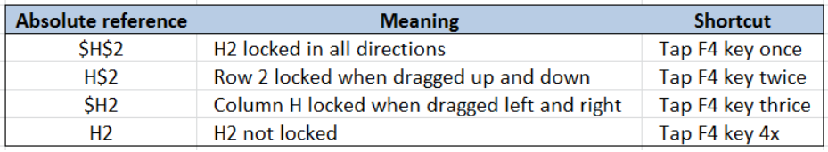 Figure 3. Dollar sign combinations in locked cells
When we tap F4 once, we lock the cell in all directions, and dollar signs appear before the column and row digits. For example, when we place the cursor on H2 in the formula below and press F4 once, H2 is locked and it will not be changed regardless of where we drag our formula.
 Figure 4. Cell locked in all directions
Tapping F4 twice will lock the cell up and down, and a dollar sign will appear before the row digit. However, dragging the formula left or right will still change the column number.
 Figure 5. Cell locked up and down
Tapping F4 three times will lock the cell left and right, and a dollar sign will appear before the column digit. However, dragging the formula up or down will still change the row number.
 Figure 6. Cell locked left and right
Trap errors in VLOOKUP and display a customized result
The errors that can be returned by VLOOKUP include #N/A, #REF! or #VALUE!. We can customize the result and prevent the display of the error values by using the IFERROR function in combination with VLOOKUP.
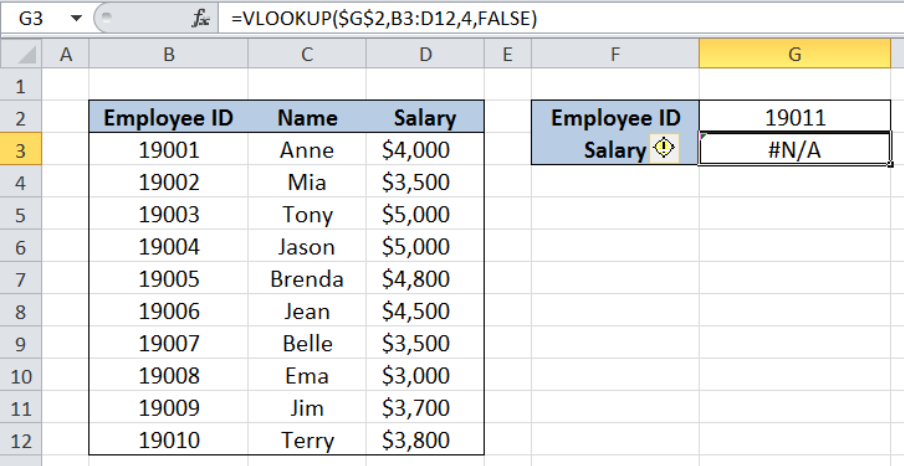 Figure 7. VLOOKUP displaying #N/A error value
We can rewrite the formula and enter this into cell G3:
=IFERROR(VLOOKUP($G$2,B3:D12,4,FALSE),"Missing Data")
 Figure 8. VLOOKUP displaying a customized result for error
With our IFERROR and VLOOKUP formula, we have replaced the error value #N/A with the text string “Missing Data”.
VLOOKUP easy to read and maintain with range names
Using named ranges makes it easy to understand and maintain our formula. Let’s take for example below formula:
=VLOOKUP(ID,Data,4,FALSE)
This formula can be easily understood where ID and Data are named ranges. ID refers to cell H2 while Data refers to the range B3:E12.
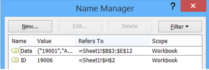 Figure 9. Name Manager preview showing named ranges
The function is looking for the exact match of the given ID in the table Data and return the corresponding value in the fourth column of Data.
Now let’s compare the formula above with this:
=VLOOKUP(H2,B3:E12,4,FALSE)
The function with named ranges is definitely easier to read. This tip is especially useful because named ranges are normally created as absolute references, which makes dragging the formula in any direction less prone to error and easy to maintain.
Use VLOOKUP to categorize data
With VLOOKUP, we can quickly categorize our data in just a few clicks.
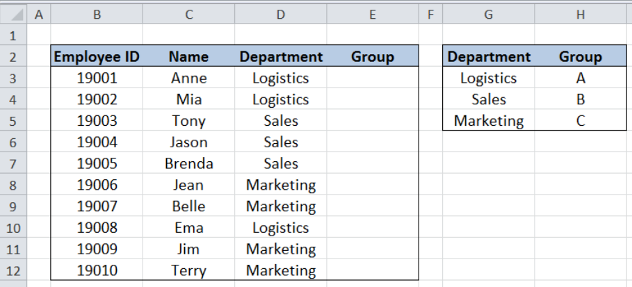 Figure 10. Sample data without group category
Suppose we have the table above consisting of four columns: Employee ID (column B), Name (column C), Department (column D) and Group (column E). In cells G3:H5, we have the data to categorize departments by group. We want to add the group category into our source table by looking up the department and finding the corresponding group.
We enter the following formula in cell E3 and drag it down to cells E4:E12:
=VLOOKUP(D3,$G$3:$H$5,2,FALSE)
With VLOOKUP, we have easily categorized the department by group for each employee in the list.
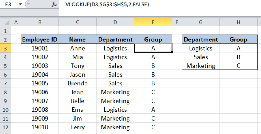 Figure 11. Data category filled up through VLOOKUP
Most of the time, the problem you will need to solve will be more complex than a simple application of a formula or function. If you want to save hours of research and frustration, try our live Excelchat service! Our Excel Experts are available 24/7 to answer any Excel question you may have. We guarantee a connection within 30 seconds and a customized solution within 20 minutes.
Are you still looking for help with the VLOOKUP function? View our comprehensive round-up of VLOOKUP function tutorials here.


Leave a Comment