Nested VLOOKUP Formula Examples

While working in VLOOKUP function in Excel, we may need to look up for values in multiple tables. This is possible by nesting VLOOKUP function. In this tutorial, we will learn how to nest VLOOKUP function in order to look up for a value.

Setting up Your Data

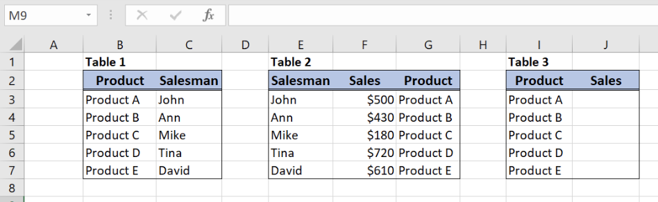Figure 1. Tables for nested VLOOKUP

We will now look at the example to explain in details how this function works. Above all, let’s start with examining the structure of the data that we will use.

The Table 1 consists of 2 columns:

• The first column is “Product” (B)
• The second one is “Salesman” (C).

The second table, Table 2, consists of 3 columns:

• Column E is “Salesman”,
• Column F is “Sales”
• While column G is “Product”.

Finally, Table 3 has 2 columns:

• Column I is “Product”
• Column J is “Sales”.

As a result, we want to get sales value in the third table (column J), depending on a product (column I).

Syntax of the VLOOKUP formula

If we want to pull the data from another table we can use VLOOKUP function. The generic formula syntax for VLOOKUP is:

=VLOOKUP(lookup_value, table_array, col_index_num, range_lookup)

The parameters of the VLOOKUP function are:

• Lookup_value– a value which we want to find in a lookup table
• Table_array– a table in which we want to look up
• Col_index_num– a column number in a lookup table from which we want to pull the data
• Range_lookup– default value 0. This means that we want to find an exact match for a lookup value.

If we try to use VLOOKUP function as in the example below, an error will appear. In VLOOKUP function table_array must be on the left side of the column from which we want to extract the data.

=VLOOKUP(I3,$F$3:$G$7,2,0)

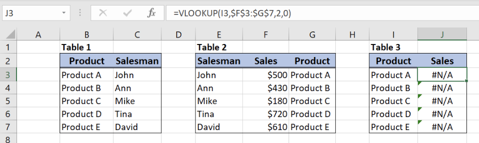Figure 2. Single VLOOKUP not working

Since single VLOOKUP function is not working, we will have to use nested VLOOKUP function:

=VLOOKUP(VLOOKUP(lookup_value1, table_array1, col_index_num1, range_lookup),table_array2, col_index_num2, range_lookup)

The nested VLOOKUP allows us to get value from a lookup table, even when we don’t have a direct relation to the main table. Therefore, we will use the second table which has a connection with both tables.

Get the Sales Values Using Nested VLOOKUP

As we can see in the picture, we don’t have a direct connection between “Product” and “Sales” columns in Table 2.In order to use VLOOKUP, the lookup column must be the leftmost.

Because of this, we will have to follow the next steps:

• First to find “Salesman” from Table 1.
• After that, we will lookup for “Sales” in Table 2 with “Salesman” from Table 1.

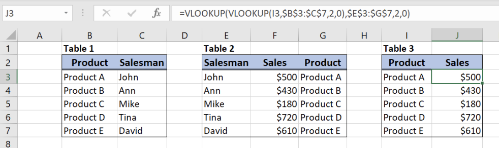Figure 3. Nested VLOOKUP formula examples

The formula looks like:

=VLOOKUP(VLOOKUP(I3,$B$3:$C$7,2,0),$E$3:$G$7,2,0)

In our example, lookup_value of the main VLOOKUP is nested VLOOKUP. We will first explain nested VLOOKUP formula part. The goal is to obtain Salesman name from the Tabel 1 who sells Product A.

Formula parts for the nested VLOOKUP will look like:

• Lookup_value – “Product A” (cell I3)
• table_array – the first table  ($B$3:$C$7)
• col_index_num2 – has value 2, as we want to pull value from the second column of the range
• range_lookup –has value 0, because we want to find an exact match of “Salesman” values

The result of this “inner” VLOOKUP will be “John” from cell C3 of the Table 1. This value will be lookup_value for the main VLOOKUP since we want to find Sales value for John in the second table.

Formula explanation for the first VLOOKUP:

• Lookup_value –nested VLOOKUP result (John)
• table_array – the second table ($E$3:$G$7)
• col_index_num2 – has value 2, as we want to pull value from the second column of the range
• range_lookup –has value 0, because we want to find an exact match of “Sales” values

To use nested VLOOKUP, we need to follow these steps:

• Select cell J3 and click on it
• Insert the formula: =VLOOKUP(VLOOKUP(I3,$B$3:$C$7,2,0),$E$3:$G$7,2,0)
• Press enter
• Drag the formula down to the other cells in the column by clicking and dragging the little “+” icon at the bottom-right of the cell.=

As a result, we will get sales $500 in the cell J3. As we can see, the value of “Salesman” for “Product A” in Table 1 is John. Therefore, the “Sales” for John in Table 2 will be $500. Finally, the VLOOKUP will return $500 in the cell B3 for “Product A”.

Most of the time, the problem you will need to solve will be more complex than a simple application of a formula or function. If you want to save hours of research and frustration, try our live Excelchat service! Our Excel Experts are available 24/7 to answer any Excel question you may have. We guarantee a connection within 30 seconds and a customized solution within 20 minutes.

Are you still looking for help with the VLOOKUP function? View our comprehensive round-up of VLOOKUP function tutorials here.