

While working with Excel, there are instances when we need to lookup a value based on multiple criteria. This can be done by modifying the lookup value in the VLOOKUP formula and modifying the source table accordingly. This step by step tutorial will assist all levels of Excel users in using VLOOKUP with multiple criteria.
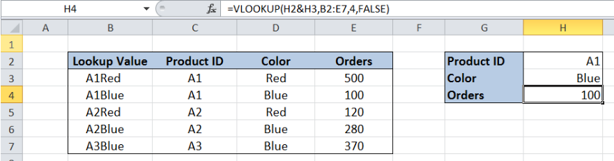 Figure 1. Final result: Use VLOOKUP with multiple criteria
Final formula: =VLOOKUP(H2&H3,B2:E7,4,FALSE)
Syntax of the VLOOKUP function
VLOOKUP is used when we want to look up and retrieve data from a given data set. To look up with multiple criteria, the syntax is:
Syntax
=VLOOKUP(lookup_value1&lookup_value2, table_array, col_index_num, [range_lookup])
The parameters of the VLOOKUP function are:
- lookup_value1 and lookup_value2: modified lookup value for VLOOKUP with multiple criteria; lookup_value1 and lookup_value2 are the values we want to search and find in the table_array; the ampersand “&” works as an AND logical operator
- table_array: the range of cells in the source table containing the data we want to retrieve
- col_index_num: the column number in the table_array corresponding to the information we want to retrieve, relative to the lookup_value
- [range_lookup]: optional; value is either TRUE or FALSE;
- if TRUE or omitted, VLOOKUP returns either an exact or approximate match
- if FALSE, VLOOKUP will only find an exact match
Setting up Our Data
Below table has four columns: “Product ID” (column B), “Color” (column C) and “Orders” (column D).
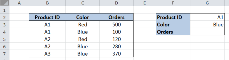 Figure 2. Sample data in using VLOOKUP with multiple criteria
In cell G4, we want to retrieve the value for orders for Product ID “1001” and Color “Blue”.
VLOOKUP in Excel is limited to handle only one lookup value, which is always in the first column of the lookup table. In order for us to lookup into two columns, we need to add a helper column in the lookup table.
We insert a column “Lookup Value” to the left of the “Product ID” column, where we link the values of columns “Product ID” and “Color”.
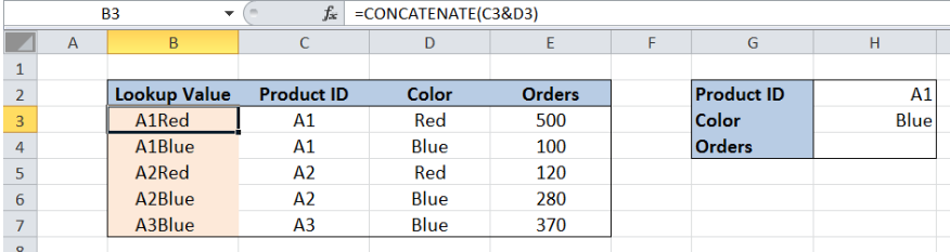 Figure 3. Modified source data in using VLOOKUP with multiple criteria
Using VLOOKUP with Multiple Criteria
We want to retrieve the value for orders for Product ID “1001” and Color “Blue”.
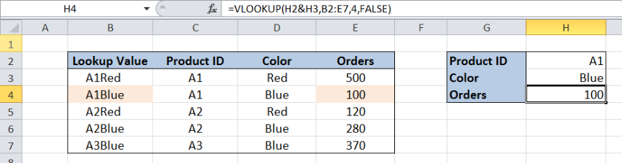 Figure 4. Entering the formula for VLOOKUP with multiple criteria
To use VLOOKUP with multiple criteria, we follow these steps:
Step 1. Select cell H4.
Step 2. Enter the formula: =VLOOKUP(H2&H3,B2:E7,4,FALSE)
Step 3. Press ENTER
For the lookup_value, we link H2 and H3 (H2&H3) using the “&” AND logical operator. The table_array is the range B2:E7. Orders is in the fourth column of the table_array so col_index_num is 4. The final result in cell H4 is 100, which is the value for Orders for Product ID 1001 with color Blue.
Most of the time, the problem you will need to solve will be more complex than a simple application of a formula or function. If you want to save hours of research and frustration, try our live Excelchat service! Our Excel Experts are available 24/7 to answer any Excel question you may have. We guarantee a connection within 30 seconds and a customized solution within 20 minutes.


Leave a Comment