How to Lock a VLOOKUP from a Table Array

By Locking the VLOOKUP from a table array, we can quickly reference a set of data against multiple lookup values. This tutorial will give you step by step instructions on how to lock the VLOOKUP table

Final formula: =VLOOKUP(D3,$A$3:$B$11,2,FALSE)

Setting up the Data

In this example the owner of Icy Treats wants to quickly know the total sales for the day. This can be achieved by using a locked VLOOKUP table array.

First, we set our data up so that the items on the menu are in Column A and the price for each item is in Column B. This will be the table array that we reference in our VLOOKUP function
Next, create another table by making Column D the items sold for the day and type this formula in cell E21 =sum(E3:E20) This will automatically add the sales prices once we calculate them with the VLOOKUP function

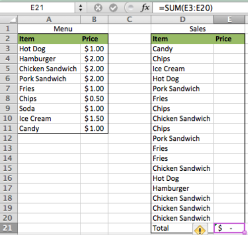Figure 1 – Setting up the data

Now all we have to do is add our VLOOKUP formula in Column E

Locking the VLOOKUP

VLOOKUP syntax: VLOOKUP(Lookup Value, Table Array, Column to Return, Approximate Match [True/False])

If we were going to be using the table for only one cell, the above syntax would work as planned. However, since we want to test the table on multiple cells, we have to add an extra factor; The Absolute Reference

An Absolute Reference can be created by typing a “$” in front of either the row or column of a cell reference. This will allow an Excel user to copy the cell reference to other cells while locking the reference point For example, take $A$1. The “$” in front of the A locks the reference to Column A and the “$” in front of the 1 locks the reference to row 1. Therefore, the reference is locked to cell A1
We can take this same approach to a set of data by creating Absolute References to the starting and ending cells of the table array
In cell E3 type this formula =VLOOKUP(D3,$A$3:$B$11,2,FALSE)
Copy the formula in cell E3 and paste it down to cell E20

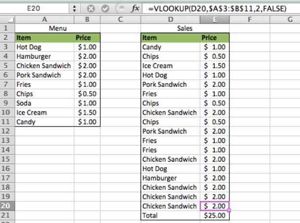Figure 2 – Locking the VLOOKUP

We can see in this example that the VLOOKUP formula quickly looked at 17 sales and returned the price for each of them by referencing only one table.

Bonus: A keyboard shortcut for creating an Absolute Reference is by pressing the F4 key on your keypad after typing the cell reference

Instant Connection to an Expert through our Excelchat Service:

Most of the time, the problem you will need to solve will be more complex than a simple application of a formula or function. If you want to save hours of research and frustration, try our live Excelchat service! Our Excel Experts are available 24/7 to answer any Excel question you may have. We guarantee a connection within 30 seconds and a customized solution within 20 minutes.

Are you still looking for help with the VLOOKUP function? View our comprehensive round-up of VLOOKUP function tutorials here.

Did this post not answer your question? Get a solution from connecting with the expert.

Another blog reader asked this question today on Excelchat:

Hello I am looking to use VLOOKUP to return certain column data out of an array. Outside of a table this is what I have been using: =VLOOKUP($B2,Sheet2!($A$8:$H$48,Column(B8),FALSE) and then dragged the formula across and down the page. This is fine, as the lookup locks to B. However, when in a table with named ranges, I cannot drag the formula across as the initial reference keep changing as I drag across. =VLOOKUP([@sampleid],[Book1]Sheet1!$A$8:$H$48,COLUMN(B8),FALSE) The initial [@sampleid] needs to be locked, I assumed with $ but nowhere i put it allows the formula to function... how do I lock this reference in a table?

An Excelchat Expert solved this problem in 18 mins!