Learn How and When to Do a VLOOKUP in Google Sheets

Syntax for the Google Sheets VLOOKUP function

VLOOKUP(search_key, range, index, [is_sorted])

Where,

Search_key – The value to be searched in the data range. It is also called lookup value or unique identifier

Range – The data table having a data set of two or more columns where data is arranged in vertical rows, and lookup values are present in the first column of a data table.

Index – The column number in a range from which data is retrieved that is related to matching lookup value in the same row.

Is_sorted – It is match type based on which you want to return lookup value; either exact match (FALSE) or approximate match (TRUE). It is optional input.

FALSE = It searches for the exact match

TRUE = It searches for an approximate match, or closest match or next smaller value than search_key, if no exact match is found. It is default match type if you omit to mention in function.

Some Points to remember

You need to remember some basic points about Google Sheets VLOOKUP

• Google Sheets VLOOKUP function is not case sensitive. It does not differentiate between uppercase and lowercase values.
• Google Sheets VLOOKUP function searches the search_key in the first column of range, leftmost column, and retrieves the information to right columns of the range.
• When is_sorted is TRUE (approximate match), then data range must be sorted in ascending order (lowest to highest) with respect to the first column of range, an otherwise VLOOKUP function may return incorrect results.
• When is_sorted is FALSE (exact match), the data range is not required to sort in any order.
• Google Sheets VLOOKUP function can search the value for a partial match using wildcard characters asterisk (*) and question mark (?). A question mark (?) is used to match any single character, but an asterisk (*) is used to match any sequence of characters.

Examples of Google Sheets VLOOKUP function

Now we will discuss some examples of Google Sheets VLOOKUP function to have more clarity on how to use this function. Suppose we have a sales data set of cigarette brands in various regions and we want to update price, sales amount and commission percentage based on sales amounts brackets.

Google Sheets VLOOKUP for Exact match

First of all, we need to update the price of each brand in the main data sheet from Price list range of each brand based on an exact match. As per above example, we have a price list of each unique brand in data range H1:I10.

When the price of each brand in each region is updated, sales amount is also updated as sales amount is the product of Quantity and Price of each carton. Google Sheets VLOOKUP for the exact match of unique Brands is as follows;

=VLOOKUP(B2,$H$1:$I$10,2,FALSE)

We need to make the range absolute by inserting $ sign with column and row references so that range reference does not change when we copy down the formula to other rows.

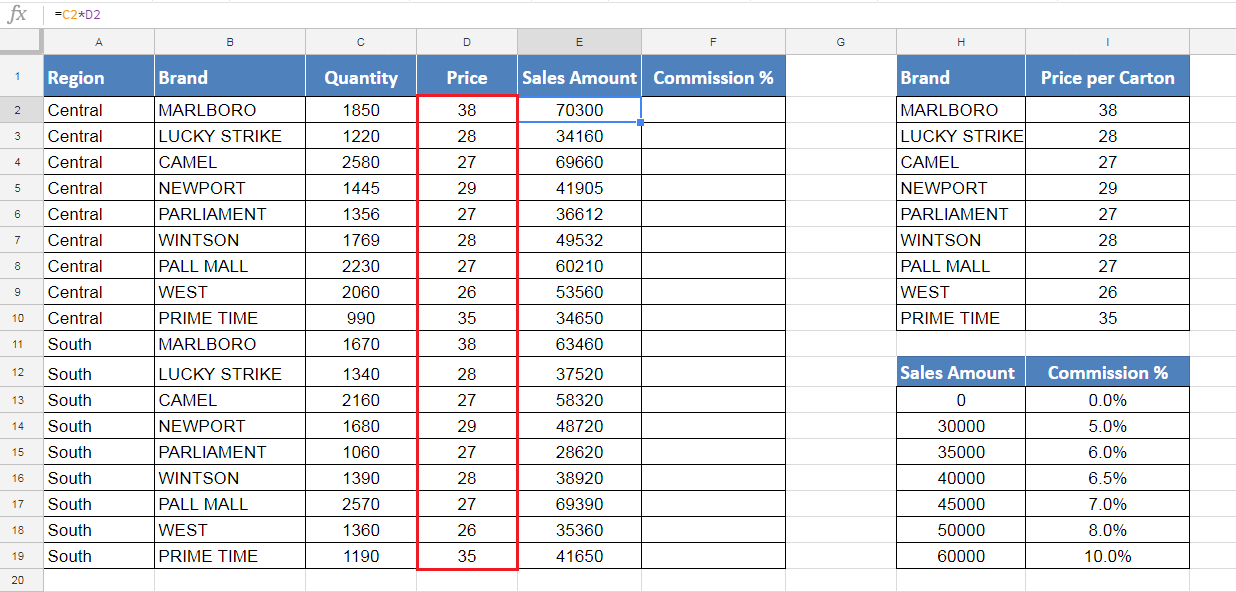
When we copy down the above Google Sheets VLOOKUP formula to other rows in Price column, it picks the price of each unique brand from Price list range. When the price of each Brand in each region is updated, the sales amount is also updated because it is a product of quantity and price as shown below;

Google Sheets VLOOKUP for approximate or closest match

Google Sheets VLOOKUP function searches the search_key based on approximate or closest match type. In this method, Google Sheets VLOOKUP formula first searches for an exact match of search_key, and if an exact match is not found then, formula looks for a value that is the closest match or next smaller value to search_key.

In this example, we need to update commission percentage (%) based on sales amount figure that we have already updated above. We have data range of commission percentage (%) with a breakup of Sales Amount. As we are going to search the value based on approximate or closest match type, so we need to sort the range (H12:I19) in ascending order by Sales Amount figures.

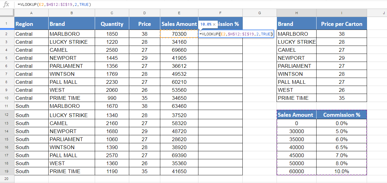
Now in column F, we need to update commission percentage based on sales amount as a search key in column E. We need to use following Google Sheet VLOOKUP formula in active cell F2 and then copy it down to other rows.

=VLOOKUP(E2,$H$12:$I$19,2,TRUE)

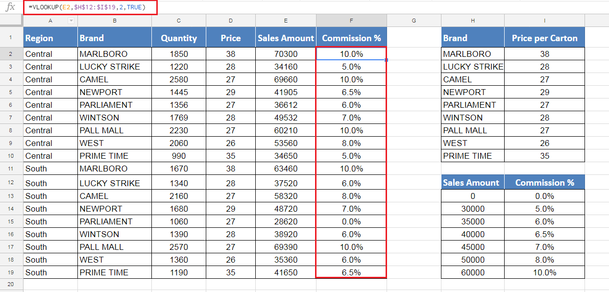
As you can see we have set the commission % based on various Sales Amount brackets, so Google Sheets VLOOKUP has picked up the commission % from the 2nd column for Sales Amount (search_key) in 1st column of range based on approximate or closest match type, where sales amount is less than or equal to search_key.