

Excel allows a user to split dimensions into two parts using several functions: SUBSTITUTE, RIGHT, LEFT, FIND and LEN. This step by step tutorial will assist all levels of Excel users to get the dimensions without units and to extract each dimension in the separate column.
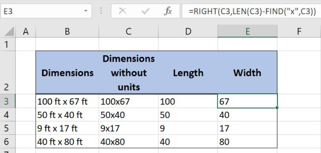 Figure 1. How to split dimensions into two parts
Syntax of the SUBSTITUTE Formula
=SUBSTITUTE(text, old_text, new_text, [instance_num])
The parameter of the SUBSTITUTE function is:
- text – a cell in which we want to substitute the text.
- old_text – a text that we want to replace
- new_text – a new text that we want to insert instead of the old text
- [instance_num] – a number of occurrences of the text that we want to replace
Syntax of the LEFT Formula
=LEFT(text, [num_chars])
The parameter of the LEFT function is:
- text – a cell from which we want to extract the characters from the left side.
- [num_chars] – a number of characters to be extracted from the left side
Syntax of the FIND Formula
=FIND(find_text, within_text, [start_num])
The parameters of the FIND function are:
- find_text – a text which we want to find in another text
- within_text -a text where we want to find a find_text
- [start_num] -a position from which we want to search for a find_text. This parameter is optional. If it’s omitted, the function will search from the beginning.
Syntax of the RIGHT Formula
=RIGHT(text, [num_chars])
The parameter of the RIGHT function is:
- text – a cell from which we want to extract the characters from the right side.
- [num_chars] – a number of characters to be extracted from the right side
Syntax of the LEN Formula
=LEN(text)
The parameter of the LEN function is:
- text – a text for which we want to count the number of characters.
Setting up Our Data for the Formula
Let’s look at the structure of the data we will use. In column B (“Dimensions”), we have dimensions with units. In column C (“Dimensions without units”), we want to get dimensions without units and spaces. In column D (“Length”) and in column E (“Width”) we want to get the dimensions from the left and from the right side of the text.
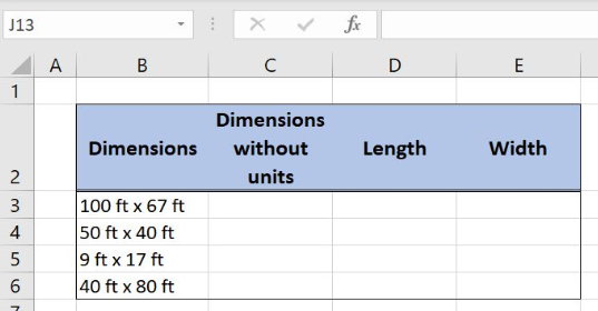 Figure 2. Data that we will use in the example
Get Dimensions Without Units
In the first step we want to get the dimensions without units and spaces from column B and to place the result in column C. For this purpose we will use SUBSTITUTE function.
The formula looks like:
=SUBSTITUTE(SUBSTITUTE(B3,"ft","")," ","")
The parameter text of the inner SUBSTITUTE function is the cell B3 with dimensions while the old_text is unit “ft” that we want to replace. The new_text is an empty space since we want to eliminate units. Finally, [instance_num] doesn’t have value because we want to replace all occurrences of the “ft” in the cell B3.
Inner SUBSTITUTE formula output has extra spaces and looks like: 100 x 67. Outer SUBSTITUTE function eliminates extra spaces from the dimensions and final formula output is 100×67, dimensions without units and spaces.
To apply the formula, we need to follow these steps:
- Select cell C3 and click on it
- Insert the formula:
=SUBSTITUTE(SUBSTITUTE(B3,"ft","")," ","") - Press enter
- Drag the formula down to the other cells in the column by clicking and dragging the little “+” icon at the bottom-right of the cell.
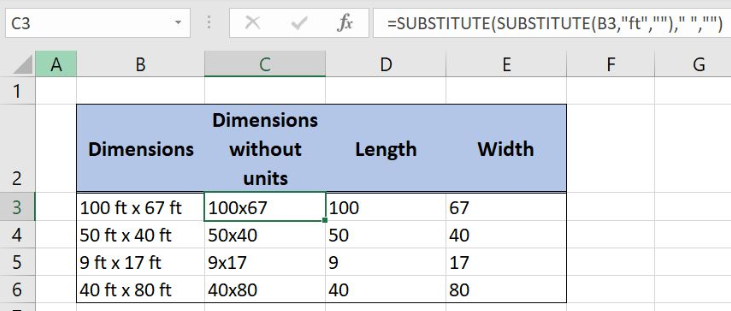 Figure 3. Get dimensions without units with SUBSTITUTE function
Extract the Left Dimension in the Separate Column
In the second step, we will extract the dimension from the left side of column C and place the number in column D.
The formula looks like:
=LEFT(C3,FIND("x",C3)-1)
The parameter text of the LEFT function is the cell C3 while the [num_chars] is the formula FIND(“x”,C3)-1. The parameter find_text in the FIND function is the string “x” while the within_text is the cell C3. The [start_num] is omitted and function will search from the beginning.
To apply the formula, we need to follow these steps:
- Select cell D3 and click on it
- Insert the formula:
=LEFT(C3,FIND("x",C3)-1) - Press enter
- Drag the formula down to the other cells in the column by clicking and dragging the little “+” icon at the bottom-right of the cell.
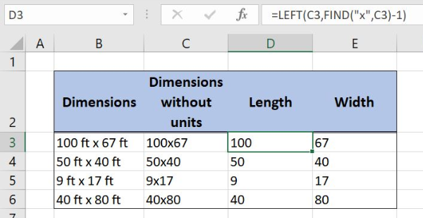 Figure 4. Extract left dimension with LEFT and FIND functions
FIND function defines a number of the characters to be extracted with the LEFT function. It returns the position of the string “x” within a cell. FIND formula output is subtracted with 1 to get the number of the characters from the left dimension. Finally, the LEFT function has the exact number of characters to be extracted from the left side and formula result is number 100.
Get the Dimension from the Right Side
Finally, we will extract the dimension from the right side of column C and place the number in column E.
The formula looks like:
=RIGHT(C3,LEN(C3)-FIND("x",C3))
The parameter text of the RIGHT function is the cell C3 while the [num_chars] is the formula LEN(C3)-FIND(“x”,C3). LEN function parameter text is the cell C3.In FIND function, find_text is the string “x” while the within_text is the cell C3. Since we want to search from the beginning, the [start_num] is omitted.
To apply the formula, we need to follow these steps:
- Select cell E3 and click on it
- Insert the formula:
=RIGHT(C3,LEN(C3)-FIND("x",C3)) - Press enter
- Drag the formula down to the other cells in the column by clicking and dragging the little “+” icon at the bottom-right of the cell.
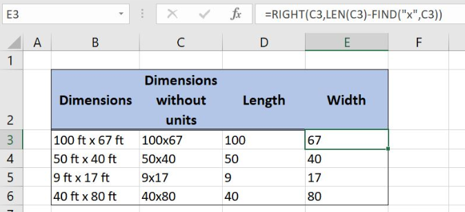 Figure 5. Get the dimension from the right
The LEN function returns the number of the characters in the cell C3 with the output 6. The result of the FIND function is number 4 because string “x” is on the 4th place in the string 100×67. When those results are subtracted we get the [num_chars] parameter of the RIGHT function. Finally, formula output is number 67, the dimension from the right side of the text.
Most of the time, the problem you will need to solve will be more complex than a simple application of a formula or function. If you want to save hours of research and frustration, try our live Excelchat service! Our Excel Experts are available 24/7 to answer any Excel question you may have. We guarantee a connection within 30 seconds and a customized solution within 20 minutes.


Leave a Comment