Excel LEFT Function

Excel allows us to get a certain number of characters from the beginning of the text, using the LEFT function. This step by step tutorial will assist all levels of Excel users in using the LEFT function.

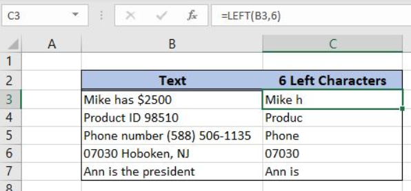Figure 1. The result of the LEFT function

Syntax of the LEFT Formula

=LEFT(text, [num_chars])

The parameters of the LEFT function are:

• text – a text from which we want to get a first part
• [num_chars] – a number of characters that we want to get from a text from the left side. This is the optional parameter, but if it is omitted, the function will return the text itself.

Setting up Our Data for Getting the Certain Number of Characters from the Beginning of the Text

Our table consists of 2 columns: “Text” (column B) and “6 Left Characters” (column C). The idea is to get the first 6 characters from column B in column C.

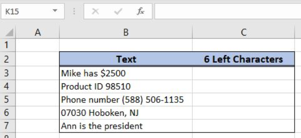Figure 2. Table structure which is used in the example

Get the Certain Number of the Characters from the Beginning of the Text

We want to get the first 6 characters from the cell B3 (“Mike has $2500”) into the cell C3.

The formula looks like:

=LEFT(B3, 6)

The text parameter is the cell B3, while the num_chars is 6. We must have in mind that the function takes into a count spaces and numbers in textual cells.

To apply the LEFT formula we need to follow these steps:

• Select cell C3 and click on it
• Insert formula: =LEFT(B3,6)
• Press ctrl, shift and enter simultaneously to create an array
• Drag the formula down to the other cells in the column by clicking and dragging the little “+” icon at the bottom-right of the cell.

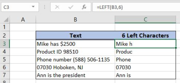Figure 3. A formula for getting the first 6 characters from the text

As you can see in Figure 3, the first 6 characters from the B3 are in the cell C3. The function counts spaces into the count, so the result in C3 is “Mike h”.

Most of the time, the problem you will need to solve will be more complex than a simple application of a formula or function. If you want to save hours of research and frustration, try our live Excelchat service! Our Excel Experts are available 24/7 to answer any Excel question you may have. We guarantee a connection within 30 seconds and a customized solution within 20 minutes.