

Excel has several built-in table styles that help us format a range of cells to be visually appealing and easy to understand. We can choose from a wide variety of table styles and even customize the created table to suit our preferences. We can also convert our table into a normal range after we are done formatting.
 Figure 1. Final result: Table styles
How to apply a table style
Suppose we have the below list of most visited countries ranked from 1 to 10, with number of visitors per country.
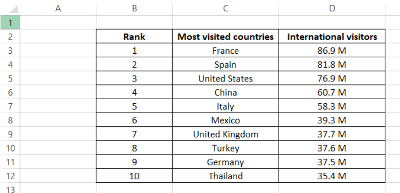 Figure 2. Sample data for Table Styles
In order to apply a table style to a range or list, we follow these steps:
- Click any cell in the range B2:D12
- Click Home tab > Format as Table on the ribbon
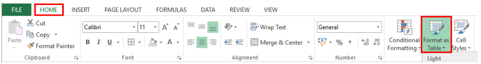 Figure 3. Format As Table menu option
- The built-in table styles will show. Let us choose Table Style Light 9.
 Figure 4. Built-in Table Styles
The Format As Table dialog box will appear, showing the range B2:D12 inside the “Where is the data for your table?” textbox. Note that Excel automatically chooses the range for our table. However, we can edit the range as we see fit.
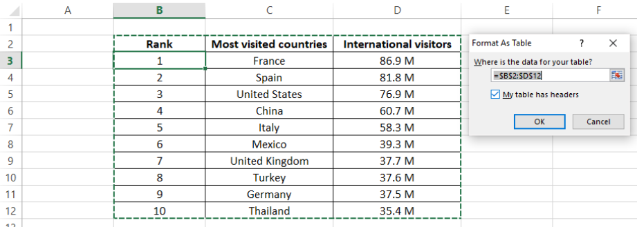 Figure 5. Format as Table dialog box
- We tick the “My table has headers” checkbox because our list has headers in row 2. Click OK.
The chosen table style will instantly apply to our table, and the Design tab under Table Tools will appear.
 Figure 6. Output: How to apply a table style
How to change table style
In order to change the table style, we click anywhere in our table and the Design tab will immediately show on the ribbon.
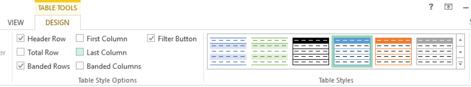 Figure 7. Table Styles in Design tab
Click the arrow at the lower right corner of the Table Styles menu to show the available table styles.
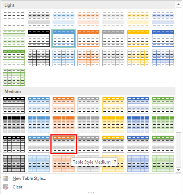 Figure 8. Table Styles menu
Let us choose Table Style Medium 17.
Our table will now reflect the new table style we selected.
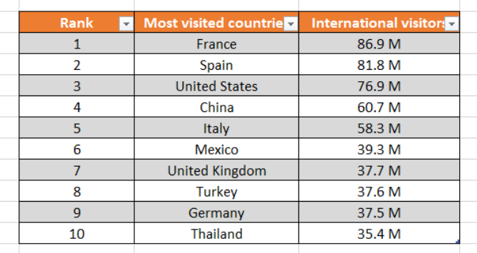 Figure 9. Output: How to change table style
How to format a table
We can further format our table by doing the following:
- Uncheck Banded Rows so that all rows have the same format
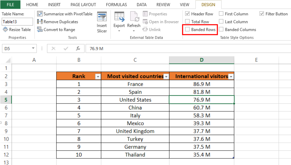 Figure 10. Output: Table with no banded rows
- Hide the filter arrows in the header by clicking anywhere on the table and selecting Filter under Home tab > Sort & Filter menu
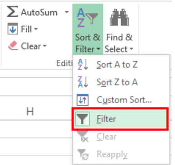 Figure 11. Filter option in Sort & Filter
This will hide the filter arrows in the row headers.
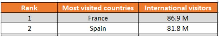 Figure 12. Output: Hide filter arrows
- Now that we have applied a table style to our list, we can opt to convert it back to a normal range, or as a normal list through these steps:
-
- Click inside the table and click Design tab > Convert to Range
- Click Yes to the prompt message: “Do you want to convert the table to a normal range?”
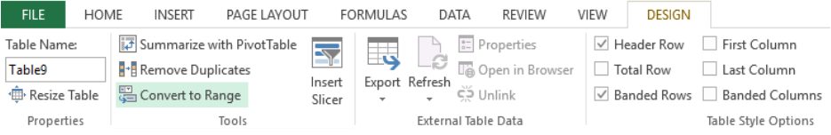 Figure 13. Convert to Range option
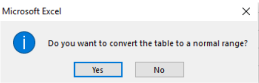 Figure 14. Convert to Normal Range prompt message
Finally, the list is now formatted as a normal range but still reflecting the table style we previously added.
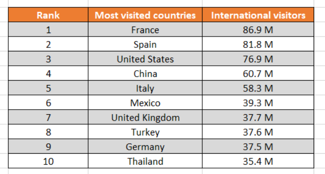 Figure 15. Output: Convert to Range
Instant Connection to an Excel Expert
Most of the time, the problem you will need to solve will be more complex than a simple application of a formula or function. If you want to save hours of research and frustration, try our live Excelchat service! Our Excel Experts are available 24/7 to answer any Excel question you may have. We guarantee a connection within 30 seconds and a customized solution within 20 minutes.


Leave a Comment