

While working with Excel, we are able to sum values that satisfy a given criteria by using the SUMIF function. This step by step tutorial will assist all levels of Excel users in summing values in cells based on background color.
 Figure 1. Final result: Using SUMIF to sum cells based on background color
Final formula: =SUMIF($D$3:$D$8,F3,$C$3:$C$8)
Syntax of the SUMIF Function
SUMIF sums the values in a specified range, based on one given criteria
=SUMIF(range,criteria, [sum_range])
The parameters are:
- Range: the data range that we will evaluate using the criteria
- Criteria: the criteria or condition that determines which cells will be added
- Sum_range: the cells that will be added; if left blank, “sum_range” = “range” which means that the range of data that will be added is the same range of data evaluated
Setting up the Data
Our table has three columns: Product ID (column B), Orders (column C) and a helper column Background Color (column D). Note that Product ID and Orders have preset background colors yellow and green.
Cells F3 and F4 contain the two background colors yellow and green, which will serve as our criteria. We want to determine the sum of the orders based on the background color. We enter the results in cells G3 and G4.
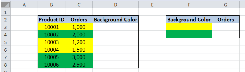 Figure 2. Sample data to sum cells based on background color
There’s no straightforward way to sum cells based on background color in Excel. For this example, the key is to assign a value for each background color, and use that value as the criteria for our SUMIF function.
Assign a number for each background color
There is a built-in function in Excel, the GET.CELL function, that returns a unique number for each background color in a cell. However, it cannot be entered directly as a worksheet function. Instead, it is used within a named range. Let us follow these steps:
Step 1. Select cells D3:D8
Step 2. Click the Formulas tab, then select Name Manager. This will launch the Name Manager dialog box.
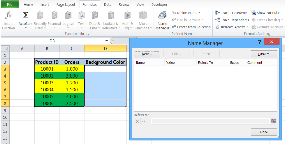 Figure 3. Create a new named range
Step 3. Click New
Step 4. In the New Name dialog box, enter “Color” for Name and the formula
=GET.CELL(38,Sheet1!C3) in the Refers to bar.
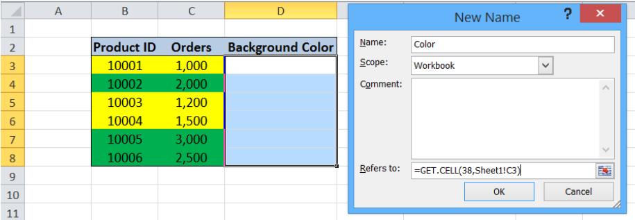 Figure 4. Entering the GET.CELL function to a new named range “Color”
This formula returns the color number unique for the background color in the adjacent cell C3.
Step 5. Click OK, then CLOSE.
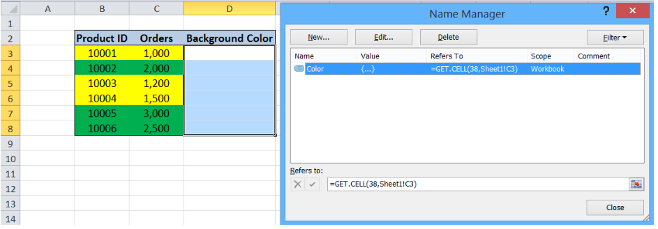 Figure 5. Named range “Color” created in Name Manager
Step 6. Select cell D3 and enter the formula: =Color
As a result, the value “6” is returned in cell D3, which is the color number for the background color yellow used in cell C3.
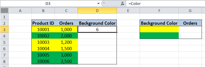 Figure 6. Assigning a number for background color of C3 using the named range “Color”
Step 7. Copy the formula in cell D3 to cells D4:D8. Below figure shows column D that is filled with the corresponding color number for the background color in column C.
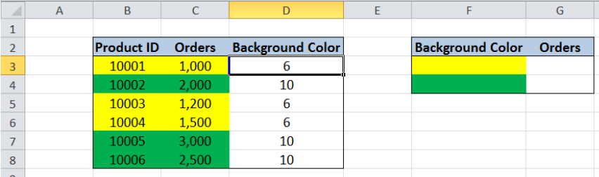 Figure 7. Assigning a number for each background color using the named range “Color”
Step 8. Enter the color number for each background color in column F: In cell F3, enter the value “6” for yellow, while in cell F4, enter the value “10” for green.
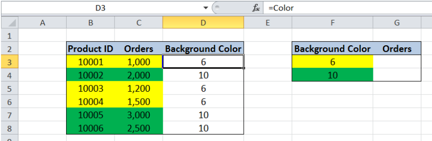 Figure 8. Assigning a number for each background color as criteria
Sum of orders based on background color
Now that each background color has a corresponding color number, we can easily sum the orders based on background color by using the SUMIF function. Let us follow these steps:
Step 1. Select cell G3
Step 2. Enter the formula: =SUMIF($D$3:$D$8,F3,$C$3:$C$8)
Step 3. Press Enter
Step 4. Copy the formula in cell G3 to cell G4.
The range we want to evaluate is D3:D8, which contains the number for the background color in column C. Our criteria in cell F3 is “6”, or the yellow color. We want to sum the orders in C3:C8 that satisfy the given criteria.
The products that satisfy our criteria and have yellow background color are cells C3, C5 and C6. As a result, the sum of orders in cell G3 is $ 3,700.
 Figure 9. Entering the formula using SUMIF to sum cells based on background color
Copying the formula in cell G3 into cell G4 returns the value $ 7,500, which is the sum of orders with green background color.
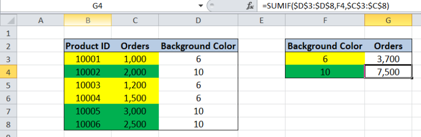 Figure 10. Output: Summing cells using SUMIF based on background color
Most of the time, the problem you will need to solve will be more complex than a simple application of a formula or function. If you want to save hours of research and frustration, try our live Excelchat service! Our Excel Experts are available 24/7 to answer any Excel question you may have. We guarantee a connection within 30 seconds and a customized solution within 20 minutes.


Leave a Comment