Sum last n columns

In Excel, we are able to sum the last n columns of any data set by using the SUM, INDEX and COLUMNS functions. The SUM function adds all given values, the INDEX function returns a value or reference to a cell, while COLUMNS returns the number of columns in an array. This step by step tutorial will assist all levels of Excel users in finding the sum of the last n columns.    

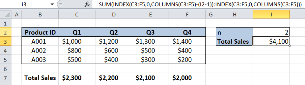Figure 1. Final result: Sum last n columns

Final formula: =SUM(INDEX(C3:F5,0,COLUMNS(C3:F5)-(I2-1)):INDEX(C3:F5,0,COLUMNS(C3:F5)))

Syntax of SUM Function

=SUM(number1,[number2],...])

• number1 – any number, array or cell reference whose values we want to add
• Only number1 is required; succeeding numbers are optional

Syntax of INDEX function

=INDEX(array, row_num, column_num)

The parameters are:

• array – a range of cells where we want to retrieve some data
• row_num – the row in the array from which we want to retrieve data
• column_num – the column in the array from which we want to retrieve data

Syntax of COLUMNS Function

=COLUMNS(array)

• array – reference to a range of cells whose number of columns we want to determine

Setting up Our Data

Our table consists of Product ID (column B) and the quarterly sales in columns C, D, E and F.  Cell I2 contains the number of columns that correspond to the last n quarters we want to sum. The resulting sum will be in cell I3.

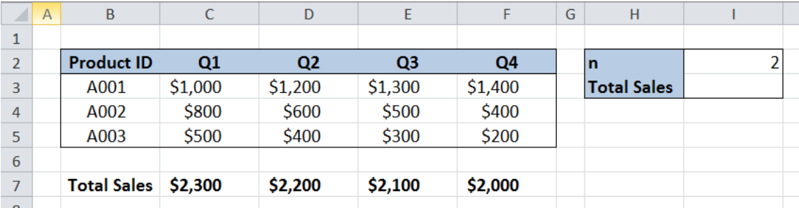Figure 2. Sample data to sum last n columns

Sum last n columns

To sum the sales for the last two quarter, we will follow these steps:

Step 1.  Select cell I3

Step 2.  Enter the formula: =SUM(INDEX(C3:F5,0,COLUMNS(C3:F5)-(I2-1)):INDEX(C3:F5,0,COLUMNS(C3:F5)))

Step 3.  Press ENTER

It is important to note that in the INDEX formula, we set the row number to zero “0” in order to lookup the entire column.  

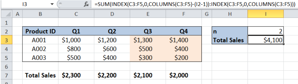Figure 3. Entering the formula to sum the last two columns

Array C3:F5 is the data range that we have.  “COLUMNS(C3:F5)” returns 4, because there are four columns in the data range.  “I2-1” returns 1 because “I2” is equal to 2.

Hence, the SUM formula is simplified and shown as an array of two INDEX formulas.  

=SUM(INDEX(C3:F5,0,3):INDEX(C3:F5,0,4))

Finally, the formula sums the third and fourth column of the range C3:F5, resulting to $4,100.  We have now successfully obtained the sum of the last two columns of our data set.

Most of the time, the problem you will need to solve will be more complex than a simple application of a formula or function. If you want to save hours of research and frustration, try our live Excelchat service! Our Excel Experts are available 24/7 to answer any Excel question you may have. We guarantee a connection within 30 seconds and a customized solution within 20 minutes.