

While working with Excel, we are able to sum values that satisfy more than one criteria by using the SUMIF, SUM and SUMPRODUCT functions. This step by step tutorial will assist all levels of Excel users in summing values that may contain either of two given criteria, employing three different methods.
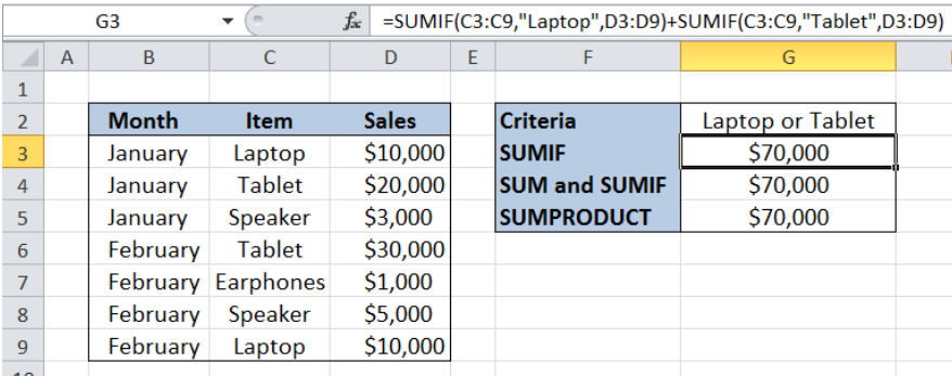 Figure 1. Final result: Sum if equal to either x or y
Formula using SUMIF : =SUMIF(C3:C9,"Laptop",D3:D9)+SUMIF(C3:C9,"Tablet",D3:D9)
Formula using SUM and SUMIF : =SUM(SUMIF(C3:C9,{"Laptop","Tablet"},D3:D9))
Formula using SUMPRODUCT : =SUMPRODUCT(D3:D9*(C3:C9={"Laptop","Tablet"}))
Syntax of the SUMIF Function
SUMIF sums the values in a specified range, based on one given criteria
=SUMIF(range,criteria, [sum_range])
The parameters are:
- Range: the data range that will be evaluated using the criteria
- Criteria: the criteria or condition that determines which cells will be added
- Sum_range: the cells that will be added; if left blank, “sum_range” = “range” which means that the range of data that will be added is the same range of data evaluated
Syntax of SUM Function
SUM adds all given values
=SUM(number1,[number2],...])
The parameters are:
- number1 – any number, array or cell reference whose values we want to add
- Only number1 is required; succeeding numbers are optional
Syntax of the SUMPRODUCT Function
SUMPRODUCT returns the sum of the products of two or more components in the given arrays
=SUMPRODUCT(array1, [array2], [array3], ...)
The parameters are:
- array – a range of values or cells whose values we want to multiply with other values and then add
- All array arguments must be in the same size
- Non-numeric values in an array are treated as zeros
Setting up the Data
Our table has three columns: Month (column B), Item (column C) and Sales (column D). Cell G2 contains our criteria “Laptop or Tablet”. We want to obtain the total sales for “Laptop” and “Tablet”. We enter the results in cells G3, G4 and G5 using three different formulas.
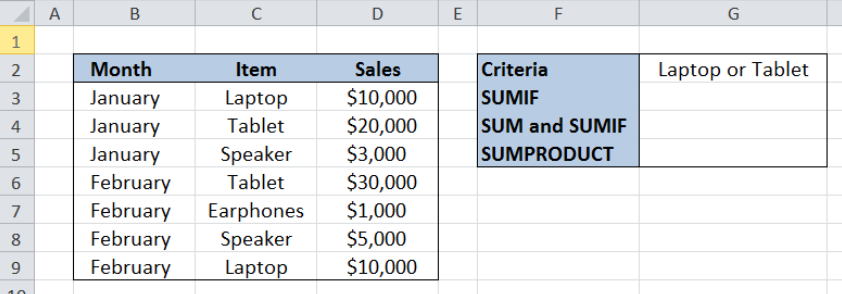 Figure 2. Sample data to sum if equal to either x or y
Sum of laptop or tablet sales using SUMIF
SUMIF function can only handle one criteria. In order to determine the sum based on two criteria, we use two SUMIF functions. Let us follow these steps:
Step 1. Select cell G3
Step 2. Enter the formula: =SUMIF(C3:C9,"Laptop",D3:D9)+SUMIF(C3:C9,"Tablet",D3:D9)
Step 3. Press Enter
The range of the data we want to evaluate is C3:C9. The are two criteria, one for each SUMIF function :“Laptop” and “Tablet”. We want to sum the sales in D3:D9 based on the given criteria.
As a result, the total sales for Laptop and Tablet in cell G3 is $70,000.
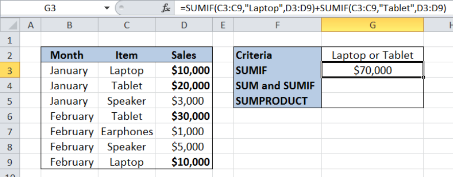 Figure 3. Using two SUMIF functions to sum sales for Laptop or Tablet
Sum of laptop or tablet sales using SUM and SUMIF
The second formula uses a combination of the SUM and SUMIF functions to sum sales based on two criteria. Let us follow these steps:
Step 1. Select cell G4
Step 2. Enter the formula: =SUM(SUMIF(C3:C9,{"Laptop","Tablet"},D3:D9))
Step 3. Press Enter
The range we want to evaluate is still C3:C9. The criteria is presented as an array inside the SUMIF function: {“Laptop“,”Tablet“}. Our formula sums the sales in D3:D9 if either of the criteria is met in C3:C9.
The final result for the total sales for Laptop and Tablet in cell G4 is $70,000, which is the same as in the previous example.
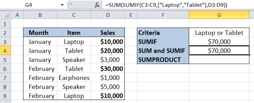 Figure 4. Using SUM and SUMIF to sum sales for Laptop or Tablet
Sum of laptop or tablet sales using SUMPRODUCT
The third formula uses the SUMPRODUCT function to sum sales based on two criteria. Let us follow these steps:
Step 1. Select cell G5
Step 2. Enter the formula: =SUMPRODUCT(D3:D9*(C3:C9={"Laptop","Tablet"}))
Step 3. Press Enter
Our third formula is somehow different because it evaluates C3:C9 based on the criteria {“Laptop“,”Tablet“} and returns as array of TRUE or FALSE for each item. The resulting array is:
{TRUE,FALSE;FALSE,TRUE;FALSE,FALSE;FALSE,TRUE;FALSE,FALSE;FALSE,FALSE; TRUE,FALSE}
SUMPRODUCT then sums the sales in D3:D9 for every TRUE result in the array.
Finally, the result in cell G5 is $70,000, which is the same as in the previous examples.
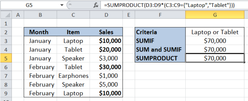 Figure 5. Using SUMPRODUCT to sum sales for Laptop or Tablet
Most of the time, the problem you will need to solve will be more complex than a simple application of a formula or function. If you want to save hours of research and frustration, try our live Excelchat service! Our Excel Experts are available 24/7 to answer any Excel question you may have. We guarantee a connection within 30 seconds and a customized solution within 20 minutes.


Leave a Comment