You can use SUMPRODUCT, MOD and COLUMN functions to filter every nth column and sum the values in those columns.

Sum every nth column

Formula

= SUMPRODUCT((MOD(COLUMN(range)-COLUMN(range.first_column)+1,N)=0)*1,range)

Explanation

Range: Required. This range includes the values you want to sum.
Range.first_column: Required. This cell locates the first column of the range.
N: Required. This help to filter Nth column in the range.

In this formula, COLUMN functions get the relative column of the range. MOD function filters if the column number is divisible by N and returns an array of TRUE/FALSE elements. Finally, SUMPRODUCT will multiply and sum the equivalent values in the range that match TRUE returns in the array. 

Example 1

Below is some of the example of using this formula. The highlighted values in the range B4:G4 help you to spot the Nth columns.

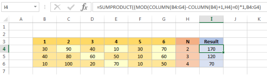
Figure 1 – Sum every nth column

In I4, the formula is

=SUMPRODUCT((MOD(COLUMN(B4:G4)-COLUMN(B4)+1,H4)=0)*1,B4:G4)

First, COLUMN(B4:G4)-COLUMN(B4)+1,H4 portion is used to get relative column number is the range. It can be seen like this in arrays: {2,3,4,5,6,7} – 2 + 1 = {1,2,3,4,5,6}
Second, MOD(COLUMN(B4:G4)-COLUMN(B4)+1,H4)=0) returns and TRUE/FALSE array to filter the column number that divisible by H4 value. The array in this case is:{FALSE,TRUE, FLASE,TRUE, FLASE,TRUE} because {2,4,6} are divisible by H4=2. Multiplying this array by 1 (*1) will return an array like this: {0,1,0,1,0,1}.

Last, SUMPRODUCT uses the above array as the argument whose components you want to add and return the result.

Notes

You can adapt this formula to sum even or odd columns like this:

=SUMPRODUCT((MOD(COLUMN(B7:G7)-COLUMN(B7)+1,2)=1)*1,B7:G7)

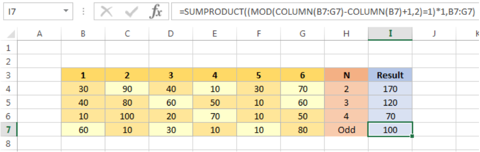
Figure 2 – Sum every odd column