While working with Excel, we are able to average values that satisfy a given criteria by using the AVERAGEIF function. This step by step tutorial will assist all levels of Excel users in the usage and syntax of AVERAGEIF function.
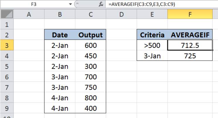
 Figure 1. Final result: Excel AVERAGEIF function
Formula 1: =AVERAGEIF(C3:C9,E3,C3:C9)
Formula 2: =AVERAGEIF(B3:B9,E4,C3:C9)
Syntax of the AVERAGEIF Function
=AVERAGEIF(range, criteria, [average_range])
- range – the data range that we will evaluate using the criteria
- criteria – the criteria or condition that determines which cells will be averaged
- average_range – optional; the cells that will be averaged; if left blank, “average_range” = “range” which means that the range of data that will be averaged is the same range of data evaluated
Setting up our Data
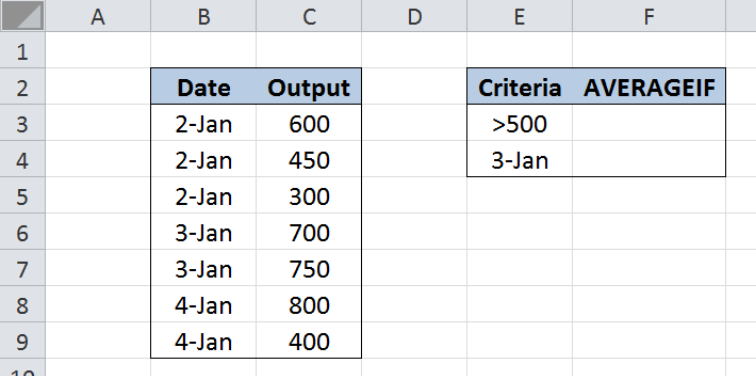
Our data consists of two columns : Date (column B) and Output (column C). In cells E3 and E4, we enter the criteria for our AVERAGEIF function. We want to calculate the average of outputs greater than 500 and the average of outputs on January 3. The results will be recorded in cells F3 and F4.
 Figure 2. Sample data for the AVERAGEIF function
Calculate the average of outputs greater than 500
We want to calculate the average of outputs greater than 500 by using the AVERAGEIF function. Let us follow these steps:
Step 1. Select cell F3
Step 2. Enter the formula: =AVERAGEIF(C3:C9,E3,C3:C9)
Step 3. Press ENTER
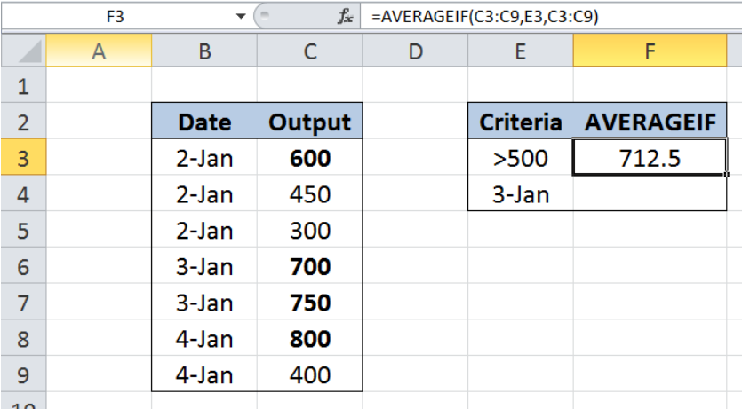
 Figure 3. Using AVERAGEIF to calculate the average of outputs > 500
The data range that we will evaluate is C3:C9. Our criteria in cell E3 is “>500”, which finds outputs greater than 500. The data range of values we want to average is also C3:C9, which contains the outputs.
As a result, our formula calculates the average of 600, 700, 750 and 800. Finally, the result in cell F3 is 712.5, which is the average of the four values.
Calculate the average of outputs on January 3
We want to calculate the average of outputs produced on January 3. Let us follow these steps:
Step 1. Select cell F4
Step 2. Enter the formula: =AVERAGEIF(B3:B9,E4,C3:C9)
Step 3. Press ENTER
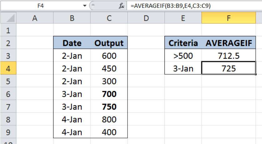
 Figure 4. Using AVERAGEIF to calculate the average output on 3-Jan
The data range that we will evaluate is B3:B9. Our criteria in cell E4 is “3-Jan”. The data range of values we want to average is C3:C9, which contains the outputs.
As a result, our formula calculates the average of 700 and 750, which are the outputs on 3-Jan. Finally, the result in cell F4 is 725, which is the average of the two values.
Notes:
- Cells that are empty, or cells containing TRUE or FALSE are ignored
- AVERAGEIF allows the use of wildcard characters such as the question mark “?” (means a single character) and asterisk “*” (means any number of characters)
- If no cells in the range meet the criteria, AVERAGEIF returns the error value #DIV/0!
Most of the time, the problem you will need to solve will be more complex than a simple application of a formula or function. If you want to save hours of research and frustration, try our live Excelchat service! Our Excel Experts are available 24/7 to answer any Excel question you may have. We guarantee a connection within 30 seconds and a customized solution within 20 minutes.


Leave a Comment