

We carry out sensitivity analysis (also called what-if analysis or data table) in Excel when we wish to observe what a specific result would look like under different conditions. We can easily select one or two variables to see the desired output. In this article, we will learn how to carry out sensitivity analysis using a Two-variable data table.
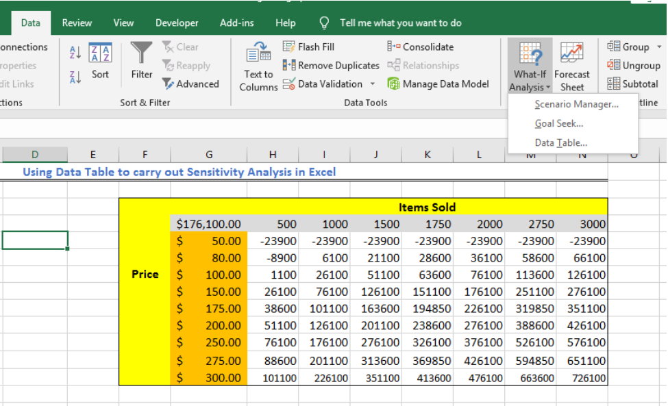 Figure 1 – Example of a sensitivity table
Two-Variable Data Table Sensitivity Analysis
We can use the data table as a shortcut to perform multiple calculations of different versions of a single scenario. It also provides a way to compare and view the results of the different variations in one place.
In this tutorial, we will create a summary of expenses and income in Columns A and B. Next, we will prepare a Profit and Loss Table, and finally, we will find the Operating Profit over different sales volumes and price of goods sold using a Sensitivity analysis table.
- First, we will create a worksheet as shown below.
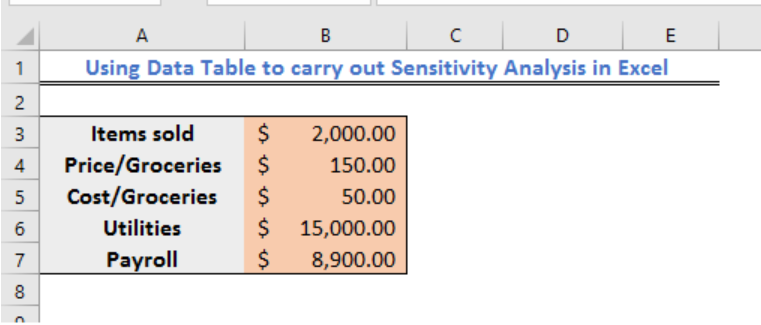 Figure 2 – Setting the items for sensitivity analysis
- Next, we will create a Profit and Loss Statement Table, where we will make our entries after the Sensitivity analysis. Where:
- In Cell B12, we will enter the formula =B4*B3;
- In Cell B13, we will enter the formula =B5*B3;
- In Cell B14, we will enter the formula =B12-B13;
- In Cell B15, we will enter the formula =B14-B6-B7.
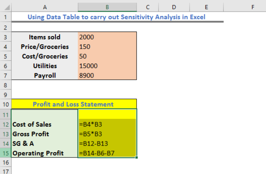 Figure 3 – How to run a sensitivity analysis
- We will have the result as shown below
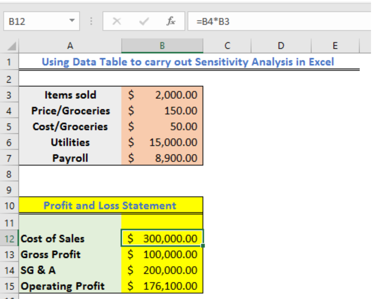 Figure 4 – Profit and loss statement for price sensitivity analysis
- Now, we will prepare our sensitivity analysis table. In the figure below, we have Price as our vertical data range while Items Sold will be our Horizontal data range.
- In Range H4:N4, we will type the Items sold (sales volumes) from 500 to 3,000
- In Range G5:G13, we will type prices from 80 to 300
- In the Cell G4, we will type the formula =B15
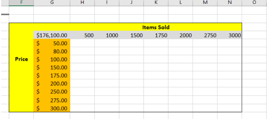 Figure 5 – Sensitivity analysis in the tutorial
- We will select Range G4:N13
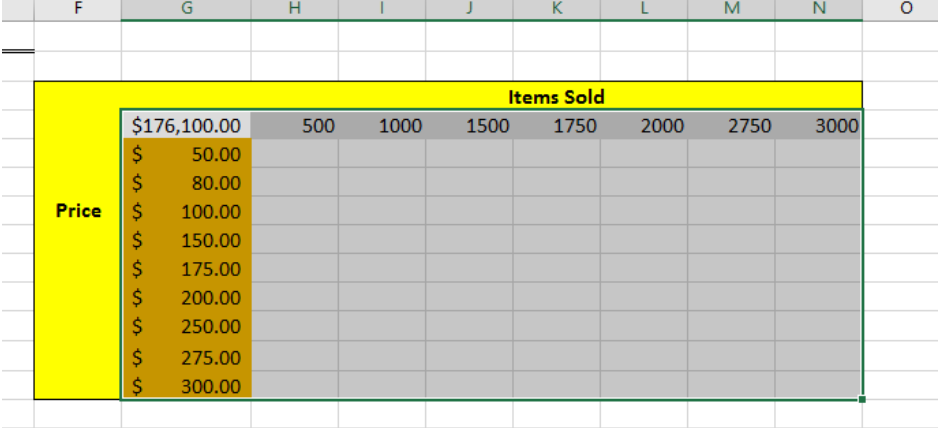 Figure 6 – Data table for sensitivity analysis
- We will go to the Data Tab, select What-If Analysis and then click on Data table
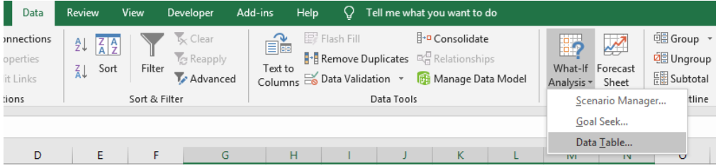 Figure 7 – How to do an excel sensitivity analysis
- In the Data table dialog box
- We will specify the cell for Items sold in the Row Input Cell box. In this case, we will enter $B$4
- We will specify the cell for Price in the Column Input Cell box. In this case, we will enter $B$5
- Lastly, we click OK.
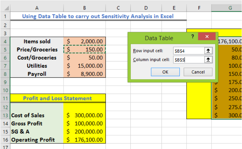 Figure 8 – Sensitivity analysis
- Once we have click OK, excel will automatically find the operating profit for each scenario.
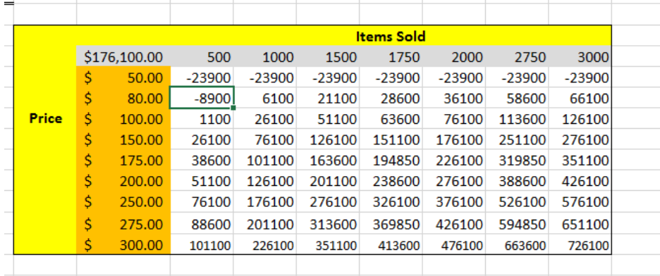 Figure 9 – Sensitivity analysis
Instant Connection to an Excel Expert
Most of the time, the problem you will need to solve will be more complex than a simple application of a formula or function. If you want to save hours of research and frustration, try our live Excelchat service! Our Excel Experts are available 24/7 to answer any Excel question you may have. We guarantee a connection within 30 seconds and a customized solution within 20 minutes.


Leave a Comment