

Testing linear regression in Excel as well as Google sheets is important, given that it might be a little hard to use other statistical tools. In this post, we shall look at how one can use find a linear regression of any model using excel and Google sheets.
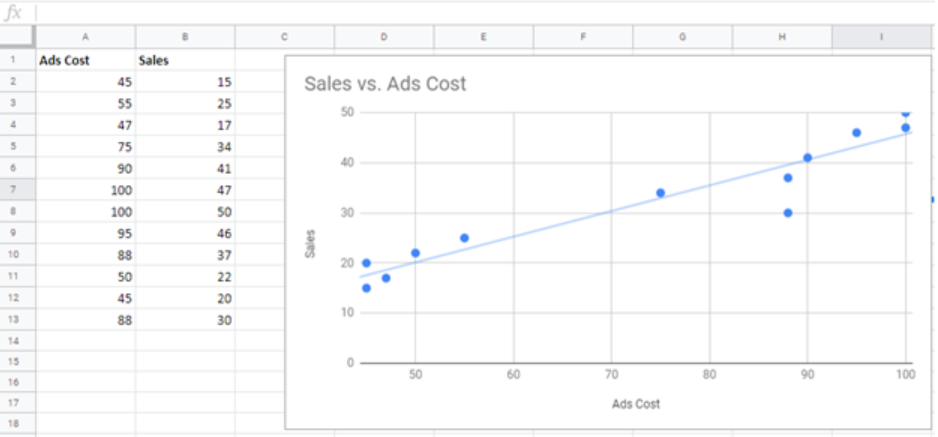 Figure 1: How to do linear regression excel
Before we start creating the linear regression line, we first need to know which data to put on the X-axis and to Y-axis. For purposes of this article, we shall use Ads Cost as the independent variable, X-axis and the sales as the dependent variable, Y-axis.
We should also be aware that a regression line simply refers to the line of best fit. This means that a straight line connecting the most number of points in the scatter graph.
Also, for purposes of this example, we shall draw our regression line in the Google sheets.
Now that we know a few basics about linear regression, let us look at a step-by-step guide on how to go about drawing this line of best fit.
Step-by-step procedure
To get a linear regression of any data, follow the steps below;
Step 1: Prepare the data
we need to have data of two variables, one being the independent and the other dependent variable. Here, we have data for advertisement costs as the independent variable and sales as values for the dependent variable.
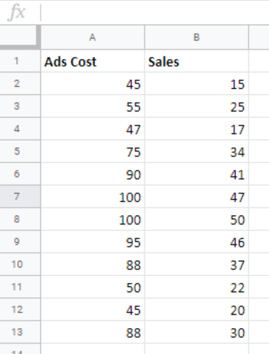 Figure 2: Linear regression data
Step 2: Highlight the data
The next thing to do is highlight the data. Left click on cell A1 and drag it down to cell B13. This will highlight the entire data. Remember that we need to highlight both the data and the labels in row 1. We need the labels so that we can put them on the vertical and horizontal axis.
Step 3: Get the scatter graph
To get linear regression excel, we need to first plot the data in a scatter graph. This is a graph that has all the points randomly put on the graph. Usually, the points are scattered all over the graph.
To get the scatter graph, click on the “Insert tab” then head to the “Chart tab”. We now need to get the scatter graph for our data. To do this, head to the insert tab and click the Chart tab.
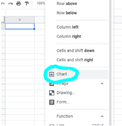 Figure 3: Selecting chart for the linear regression
Step 4: Choose scatter plot
There are many recommended charts here, but for we to plot linear regression excel, we need to scroll down and choose the scatter plot.
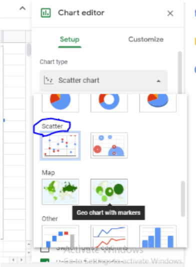 Figure 4: Choosing scatter
When we click on the scatter plot, we will have a graph with points scattered all over it. This is a scatter diagram, with all the possible points represented on it.
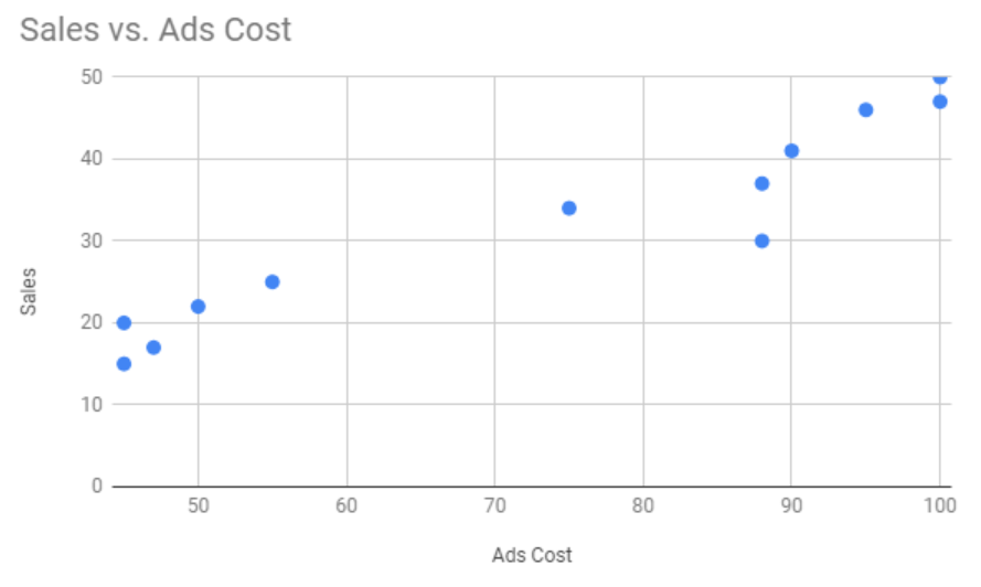 Figure 5: points on the scatter plot
Step 5: Get the trendline
After we get the scatter plot of the data, we need to check the trendline, which will help us test linear regression excel.
To get the Trendline, click the “customize tab” and then scroll down to where we have “Series”. Under series, we will be able to see the “Trendline”, check the box besides it.
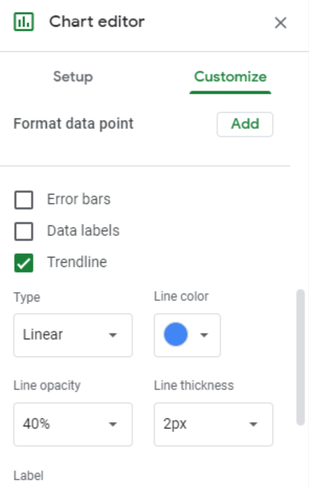 Figure 6. Trendline
Step 6: Changing the label
If we want to change the chart title and the axes labels, we can do this by selecting the “Customize tab”. Put the name that best describes wer chart under “Chart Title”. From the same point, we can also change the color of the title as well as the title font.
To change the name of the axis, we need to scroll down through the “customize” window. we will find the “Horizontal Axis” tab. Click on it and change the axis name to fit the data we have. Here, we can also change the color and font size. Do the same for the vertical axis.
Most of the time, the problem you will need to solve will be more complex than a simple application of a formula or function. If you want to save hours of research and frustration, try our live Excelchat service! Our Excel Experts are available 24/7 to answer any Excel question you may have. We guarantee a connection within 30 seconds and a customized solution within 20 minutes.


Leave a Comment