When you have a list of numbers with you, like prices, scorecard, or sales figures, and you want to get the relative position of a number from that list, then you need to use the Excel RANK function to do that. You can put the numbers in highest to lowest order (descending) or lowest to highest order (ascending) by using Excel RANK function.
How to use the RANK function in Excel
The RANK function in Excel returns the rank or order of a number within a set of numbers. Rank also refers to the size of a number relative to other numbers in the list. It is categorized as the Statistical function in Excel. It returns the same relative position for duplicate values in the list.
Syntax of the Excel RANK function is;
RANK(number,ref,[order])
Where,
Number: It is the numeric value whose rank needs to be returned.
Ref: It is a list of numbers used to rank against. It is a range or array of numbers.
Order: Optional. It specifies how to rank the numbers, whether in descending (highest to lowest) or ascending order (lowest to highest)
- If order argument is 0, the numbers are ranked in descending order.
- If the order argument is other than 0, the numbers are ranked in ascending order.
- If the order argument is omitted, Excel assumes order is 0 and numbers are ranked in descending order.
Other ways to rank numbers in Excel
Excel has two more functions to rank the numbers, introduced in Excel 2010 and later versions. It is recommended by Excel to use following two additional functions instead of a simple RANK function, which are described below, but if you are using Excel 2007 or earlier version, then only Excel RANK function is available.
RANK.EQ function in Excel returns the rank or order of a number against a list of numbers. It is the same as the RANK function in Excel, and it also returns the same rank or order of duplicate numbers in the list. The syntax of this function is the same as the RANK function.
=RANK.EQ (number, ref, [order])
RANK.AVG function returns the rank of a number against a list of other numeric values, but it returns average rank value for each of duplicate values. Its syntax is;
=RANK.AVG (number, ref, [order])
Points to Remember
- All Excel Rank functions support only numbers, positive and negative numbers, zero, date and time values. All other value types are ignored.
- All Excel RANK functions return the same rank for duplicate values and skip subsequent ranking numbers as shown in below example.
- If a number is not found within ref argument, all Excel Rank functions return #N/A
In the below example, you will learn how to use RANK, RANK.EQ and RANK.AVG function simultaneously for a set of values and see what difference between these functions is. Suppose you a list of students who have scored in a test exam, and you need to calculate the rank of each of these students in descending order, highest to lowest.
Following formulas would be used to return ranking orders using 3 Excel RANK functions;
=RANK(B2,$B$2:$B$8,0)
=RANK.EQ(B2,$B$2:$B$8,0)
=RANK.AVG(B2,$B$2:$B$8,0)
As you can see Excel RANK function and RANK.EQ function has returned the same results for unique score numbers and for duplicates as well, but RANK.AVG function has assigned an average rank score for duplicate records. All three functions have skipped sequential ranking number as the 3rd ranking position has not been assigned to any score number.
Rank Numbers Uniquely in Excel
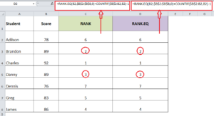
As discussed earlier that Excel RANK function assigns the same ranking position for duplicate values and skips sequential ranking number, but there could be a situation where you want to break the tie and rank uniquely each number without skipping the sequential ranking number. In order to do that you can rank duplicate values uniquely in descending order by using Excel RANK function or RANK.EQ function combined with COUNTIF function in the following formula;
=RANK(B2,$B$2:$B$8,0)+COUNTIF($B$2:B2,B2)-1
OR
=RANK.EQ(B2,$B$2:$B$8,0)+COUNTIF($B$2:B2,B2)-1

Still need some help with Excel formatting or have other questions about Excel? Connect with a live Excel expert here for some 1 on 1 help. Your first session is always free.


Leave a Comment