

Excel allows us to create a random pairing generator using the RAND, RANK, TEXTJOIN and CEILING functions. This step by step tutorial will assist all levels of Excel users to learn how to make a random pairing generator in Excel
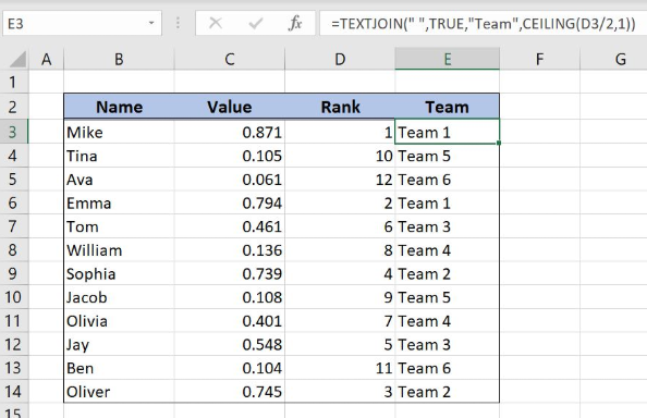 Figure 1. The final result of the formula
Syntax of the RAND Formula
=RAND()
The function returns a random decimal number between 0 and 1 and has no parameters.
Syntax of the RANK Formula
=RANK(number, ref, [order])
The parameters of the RANK function are:
- number – a number which we want to rank
- ref – a list of numbers for ranking
- [order] – 1 for ascending or 0 for descending order. This parameter is optional, if it’s omitted, the default order is descending.
Syntax of the TEXTJOIN Formula
=TEXTJOIN(delimiter, ignore_empty, text1, [text2], ...)
The parameters of the TEXTJOIN function are:
- delimiter – a string that will be used as a separator between the text items
- ignore_empty – TRUE for ignoring empty cells
- text1, [text2] – text strings that will be joined.
Syntax of the CEILING Formula
=CEILING(number, significance)
The parameters of the RANK function are:
- number – a number which we want to round up to the nearest significance
- significance – a significance for rounding a number up.
Setting up Our Data for the Formula
Let’s look at the data that we will use in the example. To group names into teams, we will need to have several helper columns. In column B (“Name”), we have names of team members. In column C (“Value”), we will have a random number 0-1 for every name. In column D (“Rank”), we will get a rank for every random number. Finally, in column E (“Team”), we’ll get the team for each name.
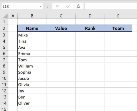 Figure 2. The data structure that we will use in the example
Set up a Random Pairing Generator
First, we need to get a random number in column C for each name.
The formula for RAND in C3 looks like:
=RAND()
To apply the formula, we need to follow these steps:
- Select cell C3 and click on it
- Insert the formula:
=RAND() - Press enter
- Drag the formula down to the other cells in the column by clicking and dragging the little “+” icon at the bottom-right of the cell.
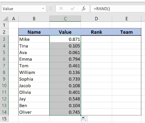 Figure 3. Using the RAND formula
When we get a random number for each name we can rank them in column D.
The formula for RANK in D3 looks like:
=RANK(C3, $C$3:$C$14)
The number parameter is the cell C3. The ref parameter is the range $C$3:$C$14. We must fix the range, as it’s not changing when the formula is copied down the cells.
To apply the formula, we need to follow these steps:
- Select cell D3 and click on it
- Insert the formula:
=RANK(C3,$C$3:$C$14) - Press enter
- Drag the formula down to the other cells in the column by clicking and dragging the little “+” icon at the bottom-right of the cell.
![]() Figure 4. Using the RANK formula
Figure 4. Using the RANK formula
Now we have the rank for every random number in column D and can divide them by 3.
Finally, we can use the TEXTJOIN and CEILING formula, to assign team pairs to each name. Using the TEXTJOIN we will just concatenate “Team” and team number, while using the CEILING we will get the team number for each name.
The formula for TEXTJOIN and CEILING in E3 looks like:
=TEXTJOIN(" ", TRUE, "Team", CEILING(D3/2, 1))
The parameter number of the CEILING function is the cell D3/2, while the significance is 1. The result of the CEILING function is the text2 parameter of the TEXTJOIN function. The text1 is “Team”, the delimiter is a space “ “ and the ignore_empty is TRUE.
To apply the formula, we need to follow these steps:
- Select cell E3 and click on it
- Insert the formula:
=TEXTJOIN(" ", TRUE, "Team", CEILING(D3/2, 1)) - Press enter
- Drag the formula down to the other cells in the column by clicking and dragging the little “+” icon at the bottom-right of the cell.
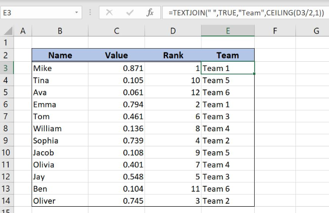 Figure 5. Using the TEXTJOIN and CEILING formula
As you can see in Figure 6, in “Team” column we have assigned a team for each name from column B and every team has two members.
Most of the time, the problem you will need to solve will be more complex than a simple application of a formula or function. If you want to save hours of research and frustration, try our live Excelchat service! Our Excel Experts are available 24/7 to answer any Excel question you may have. We guarantee a connection within 30 seconds and a customized solution within 20 minutes.


Leave a Comment