

Excel allows us to create a randomized list using the CHOOSE and RANDBETWEEN functions. This step by step tutorial will assist all levels of Excel users to learn how to create a randomized list in Excel.
 Figure 1. The final result of the formula
Syntax of the RANDBETWEEN Formula
The generic formula for the RANDBETWEEN function is:
=RANDBETWEEN(bottom, top)
The parameters of the RANDBETWEEN function are:
- bottom – a value from which we want to get a random value
- top – a value to which we want to get a random value.
Syntax of the CHOOSE Formula
The generic formula for the CHOOSE function is:
=CHOOSE(index_num, value1, [value2], [value3],...)
The parameters of the CHOOSE function are:
- index_num – an index of the value which we want to retrieve
- value1, [value2], [value3],… – a list of values from which one value is returned.
Create a Randomized List Using the Formula
In column B, we want to get a randomized list of 5 from the following items: “Computer”, “Telephone”, “Monitor”, “Keyboard”, “Mouse”.
The formula looks like:
=CHOOSE(RANDBETWEEN(1,5), "Computer", "Telephone", "Monitor", "Keyboard", "Mouse")
The parameter bottom of the RANDBETWEEN function is 1 and the top is 5. The result of this function is a random number between 1 and 5 which is the index_num parameter of the CHOOSE function. The values of the function are “Computer”, “Telephone”, “Monitor”, “Keyboard”, “Mouse”.
To apply the formula, we need to follow these steps:
- Select cell B3 and click on it
- Insert the formula:
=CHOOSE(RANDBETWEEN(1,5), "Computer", "Telephone", "Monitor", "Keyboard", "Mouse") - Press enter
- Drag the formula down to the other cells in the column by clicking and dragging the little “+” icon at the bottom-right of the cell.
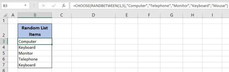 Figure 2. Using the formula to get a randomized list
If we evaluate the function in B3, we can see that the RANDBETWEEN function returns number 1. Therefore, the CHOOSE function returns the first value from the values. Finally, the result in the B3 cell is “Computer”. When we copy the formula down to the other cells, we get the randomized list of values.
Most of the time, the problem you will need to solve will be more complex than a simple application of a formula or function. If you want to save hours of research and frustration, try our live Excelchat service! Our Excel Experts are available 24/7 to answer any Excel question you may have. We guarantee a connection within 30 seconds and a customized solution within 20 minutes.


Leave a Comment