

Excel allows a user to generate a random number in a table using the INDEX, RANDBETWEEN and ROWS functions. This step by step tutorial will assist all levels of Excel users to discover how to generate a random number in a table in Excel.
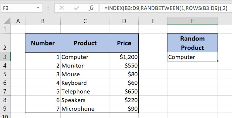 Figure 1. The final result of the formula
Syntax of the INDEX formula
The generic formula for the INDEX function is:
=INDEX(array, row_num, column_num)
The parameters of the INDEX function are:
- array – a range of cells where we want to get a data
- row_num – a number of a row in the array for which we want to get a value
- column_num – a column in the array which returns a value.
Syntax of the RANDBETWEEN Formula
The generic formula for the RANDBETWEEN function is:
=RANDBETWEEN(bottom, top)
The parameters of the RANDBETWEEN function are:
- bottom – a value from which we want to get a random value
- top – a value to which we want to get a random value.
Syntax of the ROWS formula
The generic formula for the ROWS function is:
=ROWS(array)
The parameter of the ROWS function is:
- array – a range of cells which rows we want to count.
Setting up Our Data for the Example
Let’s look at the structure of data that we will use. In the table, we have 3 columns: “Number” (column B), “Product” (column C) and “Price” (column D). In the cell F3, we want to get a random product from the table B3:D9.
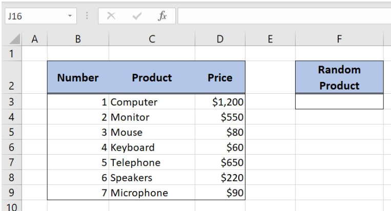 Figure 2. Data that we will use in the example
Generate a Random Value from the Table
We want to get a random product from column C of the table in the cell F3.
The formula in F3 looks like:
=INDEX(B3:D9, RANDBETWEEN(1, ROWS(B3:D9)), 2)
The parameter array of the ROWS function is the range B3:D9. The result of the ROWS function is the top parameter of the RANDBETWEEN function, while the bottom is 1. This function returns a random row number of a table. This is the row_num parameter of the INDEX function. The array parameter is B3:D9, while the column_num is 2, as we want to get a value from the second column of the table.
To apply the formula, we need to follow these steps:
- Select cell F3 and click on it
- Insert the formula:
=INDEX(B3:D9,RANDBETWEEN(1,ROWS(B3:D9)),2) - Press enter.
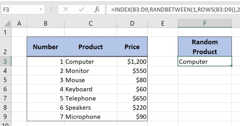 Figure 3. Using the formula to generate a random value from a table
The ROWS function returns 7, as our table has 7 rows. Therefore, the RANDBETWEEN returns a random number between 1 and 7, in our case 1. Finally, the INDEX function returns the value from row 1 and column 2 of the table. The result in the cell F3 is “Computer”.
Most of the time, the problem you will need to solve will be more complex than a simple application of a formula or function. If you want to save hours of research and frustration, try our live Excelchat service! Our Excel Experts are available 24/7 to answer any Excel question you may have. We guarantee a connection within 30 seconds and a customized solution within 20 minutes.


Leave a Comment