How to Sort Data in a Pivot Table

Excel allows us to sort data in a Pivot table in several ways. This step by step tutorial will assist all levels of Excel users in sorting data in a Pivot Table using standard Excel sort or Pivot sort option.

Figure 1. Final result

Setting up Our Data for Sorting Data in a Pivot Table

Our table consists of 3 columns: “Salesman” (column A), “Month” (column B) and “Sales” (column C). In the Pivot, table we want to get Total sales per Salesman and Month.

Figure 2. Data that we will use for the Pivot table creation

In our example, we create the Pivot table from our data.

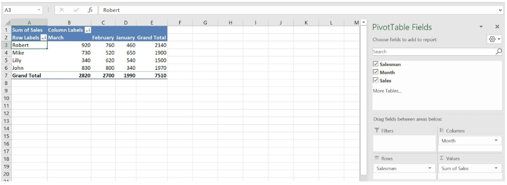Figure 3. The Pivot table

Sorting Data in the Pivot Table with Standard Excel Sort

The first way to sort data in the Pivot table is to use the standard Excel option for sorting in the Home tab. If we want to sort the table ascending by Row labels (Salesman), we need to click on any value in the Row labels, then click on Sort & Filter option in Home tab and Sort A to Z:

Figure 4. Sorting the Pivot table by Row Labels using the standard Excel sorting

As a result, the table is sorted by Salesmen in alphabetical order from A to Z:

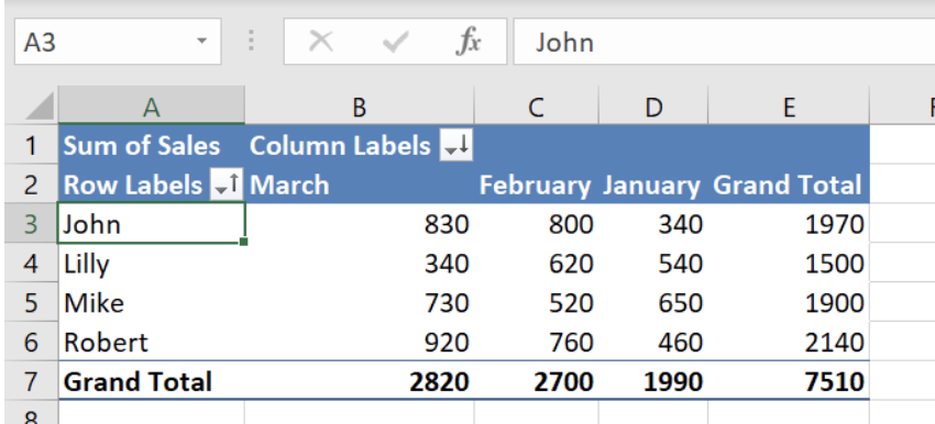Figure 5. The Pivot table sorted ascending by Salesmen

Similarly, if we want to sort the Pivot table ascending by Column labels (Months), we need to click on any value in the Column labels, then click on Sort & Filter option in Home tab and Sort A to Z:

Figure 6. Sorting the Pivot table by Column Labels using the standard Excel sorting

As a result, the table is sorted by Months in alphabetical order from A to Z:

Figure 7. The Pivot table sorted ascending by Months

Sorting Data in the Pivot Table with Pivot AutoSort

Another way to sort data in the Pivot table is to use the AutoSort option in the Pivot table. If we want to sort the table ascending by Row labels (Salesman), we need to click on the AutoSort icon next to the Row Labels, choose Sort A to Z and click OK:

Figure 8. Sorting the Pivot table by Row Labels using the AutoSort Pivot option

As a result, the table is sorted by Salesmen in alphabetical order from A to Z:

Figure 9. The Pivot table sorted ascending by Months

Similarly, if we want to sort the Pivot table ascending by Column labels (Months), we need to click on the AutoSort icon next to the Column Labels, choose Sort A to Z and click OK:

Figure 10. Sorting the Pivot table by Column Labels using the standard Excel sorting

As a result, the table is sorted by Months in alphabetical order from A to Z:

Figure 11. The Pivot table sorted ascending by Months

Most of the time, the problem you will need to solve will be more complex than a simple application of a formula or function. If you want to save hours of research and frustration, try our live Excelchat service! Our Excel Experts are available 24/7 to answer any Excel question you may have. We guarantee a connection within 30 seconds and a customized solution within 20 minutes.