

Excel Pivot Table is a very handy tool to summarize and analyze a large dataset. The Pivot Table has many built-in calculations under Show Values As menu to show percentage calculations. In a sales dataset of different cigarettes brands in various regions, we want to learn how to show Pivot Table percentages instead of Totals to compare amounts in calculations.
 Figure 1. Pivot Table Calculations
Percentage of Grand Total
In Pivot Table percentages we use % of Grand Totals calculation to compare each value to the grand total value. In our Pivot Table, Brands are placed in the Row area, Regions in the Column area and Sales Amounts in Value area. We want to show the percentage of each brand’s sales in each region while comparing with the overall Sales of all the brands across all the regions. We do the followings to change to sales amount of each brand as % of Grand Total:
- Right click on any of the brand’s sales amount cells
- Click on Show Values As
- Select % of Grand Total
 Figure 2. Selecting % of Grand Total
 Figure 3. Showing % of Grand Total
Percentage of Column Total
The percentage of Column Total calculation is used to compare each value with the total of a column value and show as the percentage of column total in Pivot Table percentages. In our Pivot table, do the following steps to show the percentage of sales for each brand within each region:
- Right click on any of the brand’s sales amount cells
- Click on Show Values As
- Select % of Column Total
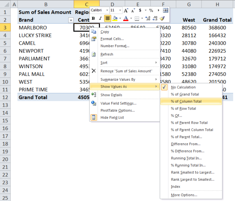 Figure 4. Selecting % of Column Total
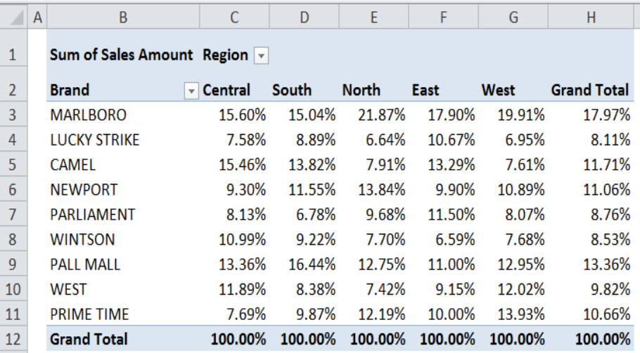 Figure 5. Showing % of Column Total
Percentage of Row Total
The percentage of Row Total in Pivot Table percentages compares each value of a row with the total value of that row and shows as the percentage. In our Pivot table, do the following steps to show the percentage of sales for each region across each brand row:
- Right click on any of the brand’s sales amount cells
- Click on Show Values As
- Select % of Row Total
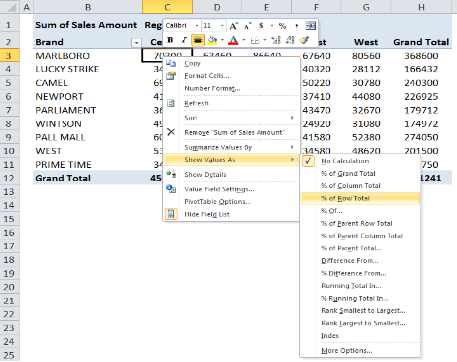 Figure 6. Selecting % of Row Total
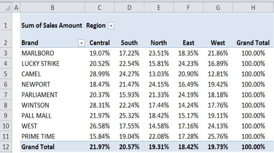 Figure 7. Showing % of Row Total
Instant Connection to an Expert through our Excelchat Service
Most of the time, the problem you will need to solve will be more complex than a simple application of a formula or function. If you want to save hours of research and frustration, try our live Excelchat service! Our Excel Experts are available 24/7 to answer any Excel question you may have. We guarantee a connection within 30 seconds and a customized solution within 20 minutes.


Leave a Comment