

We can format Pivot Tables in several ways like refreshing the table when we have new data, doing number formatting, and designing the Pivot Table. The steps below will walk through the process.
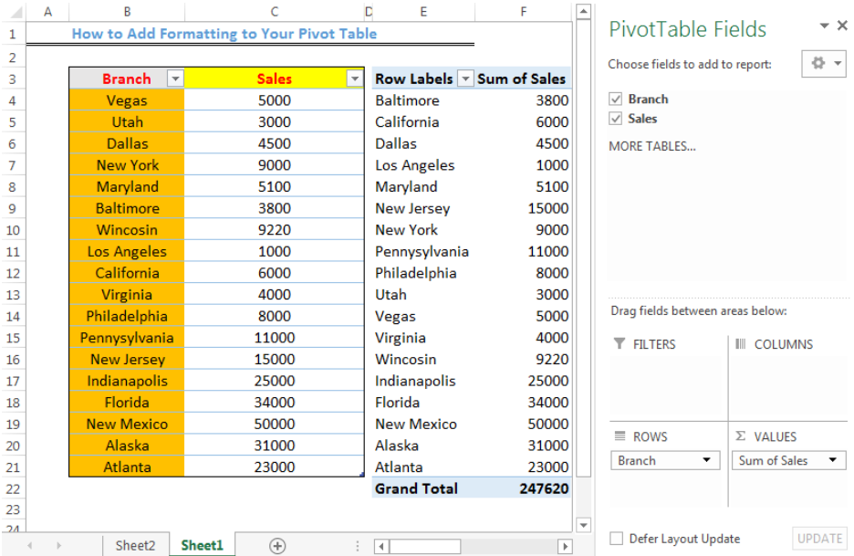 Figure 1: Refreshed Pivot Table with New Data
Setting up the data
- We will use the Pivot Table in figure 2 to illustrate how we will format our Pivot Table
 Figure 2: Setting up the Data
Refreshing the Pivot Table
We need to refresh our Pivot Table whenever we add new data to the data table.
- We can expand the Range of the Table by taking our cursor to the edge as shown in figure 3 and drag down
 Figure 3: Expanding the Range of the Data Table
- We will insert new values into the empty cells
 Figure 4: Values inserted into the Expanded Range of the Data Table
- Our Pivot Table doesn’t automatically update as we add these values
- We will click on the Pivot Table, right-click, and click on Refresh
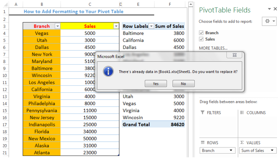 Figure 5: Prompt to Replace the Pivot Table
- We will click Yes since we want to update the current Pivot table
 Figure 6: Refreshed Pivot Table with New Data
Number Formatting
- We can format the Sum of Sales in figure 6 to have a particular currency like the United States Dollar ($)
- We will click on any cell of the Sum of Sales Column
- We will right-click and click on Number format
 Figure 7: Format Cells Dialog Box
- We will click on Currency and set the decimal places to 0. We will also set the symbol as $
- We will click OK
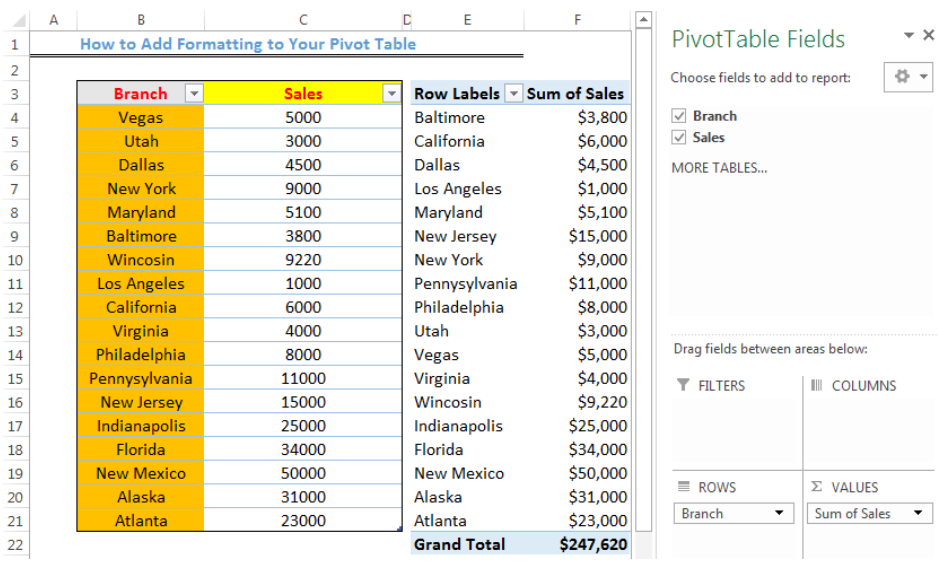 Figure 8: Formatted Cells with Currency ($)
Pivot Table Designs
- We can design our Pivot Table by clicking on the Pivot table to have access to the Pivot table tools
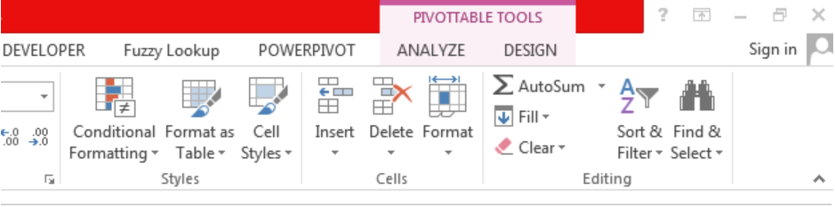 Figure 9: Pivot Table Tools
We will click on Design
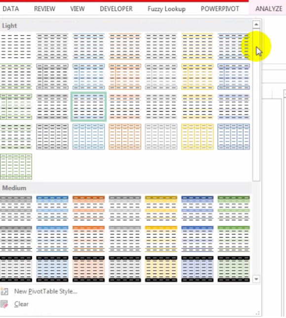 Figure 10: Design styles for our Pivot Table
- We will click on our choice
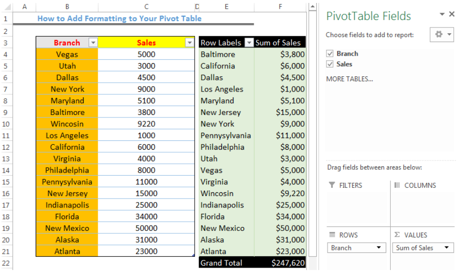 Figure 11: Designed Pivot Table
- With the Design tab, we can also alter the subtotals and grand totals by clicking on the drop-down arrow
 Figure 12: Pivot Table tool for altering Subtotals and Grand totals
Instant Connection to an Expert through our Excelchat Service
Most of the time, the problem you will need to solve will be more complex than a simple application of a formula or function. If you want to save hours of research and frustration, try our live Excelchat service! Our Excel Experts are available 24/7 to answer any Excel question you may have. We guarantee a connection within 30 seconds and a customized solution within 20 minutes.


Leave a Comment