Here is Why Your Next Pivot Table Should Have a Dynamic Range

We usually use pivot tables to help analyze and simplify massive amount of data.  However, it gets tricky when we add or remove values in our source table, and the pivot table doesn’t automatically update.  A dynamic range solves this problem. This step by step tutorial will walk through how to use a dynamic range in Pivot Tables

Setting up the Data

Here we have a table of product orders from January to February.  

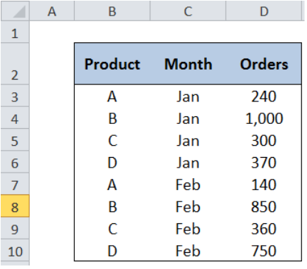Figure 1.  Data for our pivot table

Pivot Table without a Dynamic Range

First let us create a pivot table without a dynamic range, and try adding some data.  Let us see what happens to the pivot table.

Step 1. Select the range of cells that we want to analyze through a pivot table. In this case, we select cells B2:D10.  

Step 2. Click the Insert tab, then Pivot Table. This will launch the Create PivotTable dialog box.

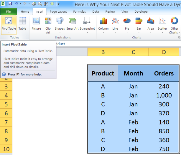Figure 2. Inserting a Pivot Table

Step 3. In the Create PivotTable dialog box, tick Existing Worksheet.  Click the bar for Location and then click cell F2. This will position the pivot table in the existing worksheet, at cell F2.

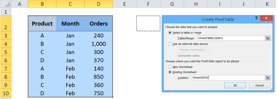Figure 3. Inserting a pivot table in an existing worksheet

Step 4. In the PivotTable Field List,  tick Product and Orders, then drag Month to the Column Labels.  This will show the Sum of Orders for each product per month.  

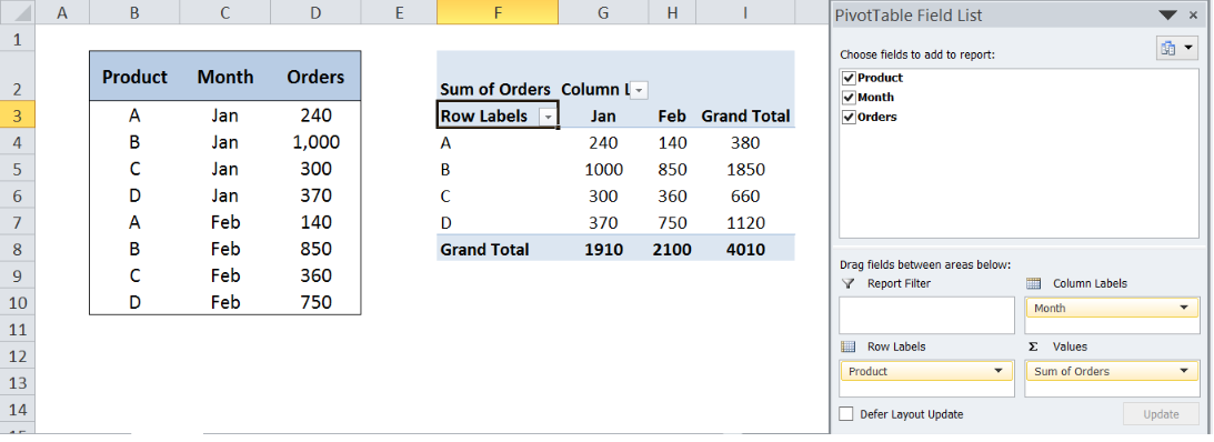Figure 4. Selecting the fields for values to show in a pivot table

Adding more data

Step 5. Now let’s add data for March in cells B11:D14.

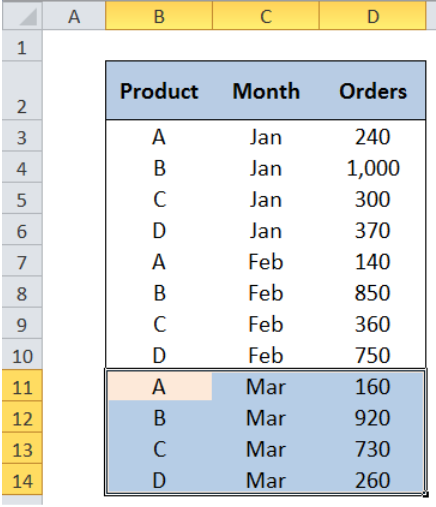Figure 5. Adding more values into our source data

Step 6. Press Ctrl + Alt + F to refresh the pivot table.  We will see that nothing happens.  Adding more data to our source table does not automatically expand our PivotTable.

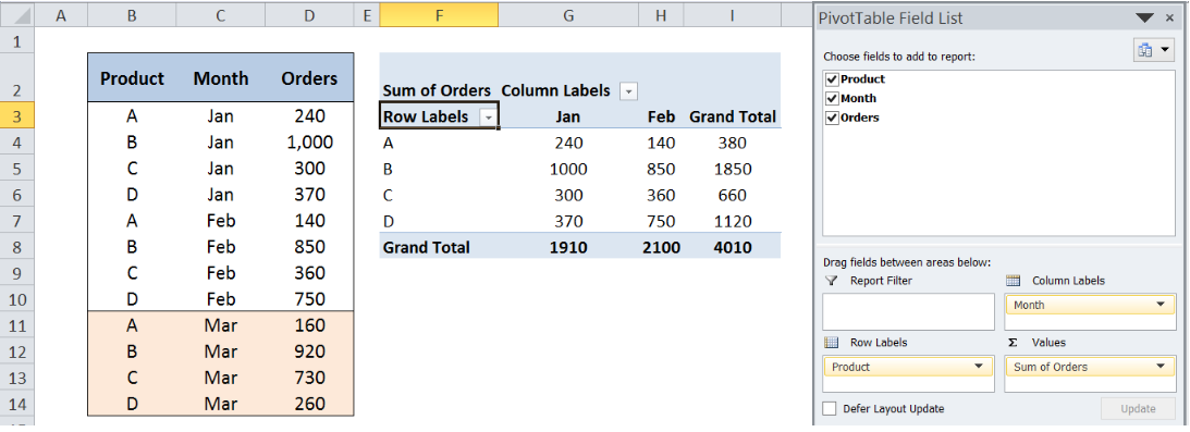Figure 6. Pivot table not updated after adding more values

Work-around:

We can change the data source to expand the data range.

Click any value in the pivot table, then click Change Data Source under the Options tab.  

Click the button beside the Table/Range bar and select cells B2:D14 to expand the data selection.   

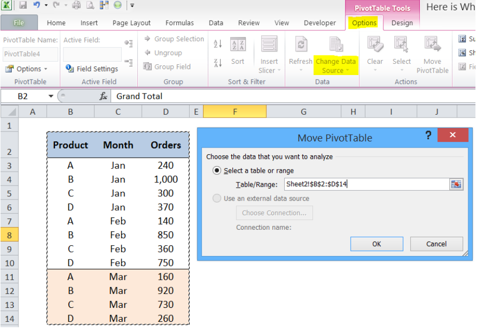Figure 7. Changing the data source for our pivot table

Click Yes to the Excel prompt message shown below:

Figure 8. Excel prompt message

The pivot table will then be updated, showing the March data.  

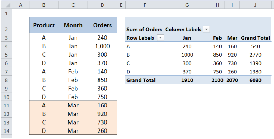Figure 9. Updated pivot table after changing the data source

Removing Data

What happens when we remove data from our table?  Let us try and delete the March data from B11:D14 and refresh by pressing Ctrl + Alt + F.  

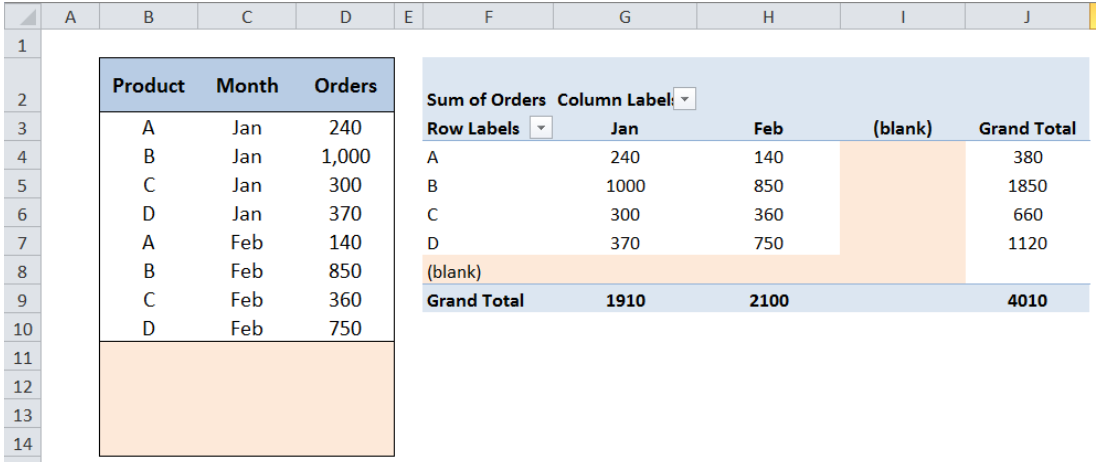Figure 10. Pivot table not updated after removing some values

The resulting pivot table does not shrink with the data.  Instead, the pivot table shows blank spaces taking the place of the deleted data.  

The complications arising from adding or removing data will be addressed by using a dynamic range in our pivot table.

Creating a Dynamic Range

We will use the same starting data as the previous example.

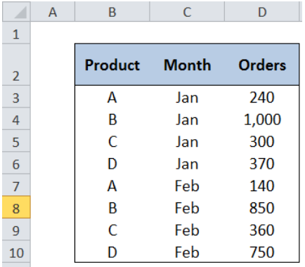Figure 11. Data for pivot table with dynamic range

One method to create a dynamic range is through the OFFSET formula.  

Syntax

=OFFSET(reference, rows, cols, [height], [width])

Where

• Reference: the reference cell for our dynamic range
• Rows: the number of rows relative to the reference cell that we want to refer to
• Cols: the number of columns relative to the reference cell that we want to refer to
• [height]: the number of rows for our dynamic range
• [width]: the number of columns for our dynamic range

Step 1. Click the Formulas tab, then select Name Manager.

Figure 12. Creating a dynamic range through Name Manager

Step 2. In the Name Manager dialog box, click New.

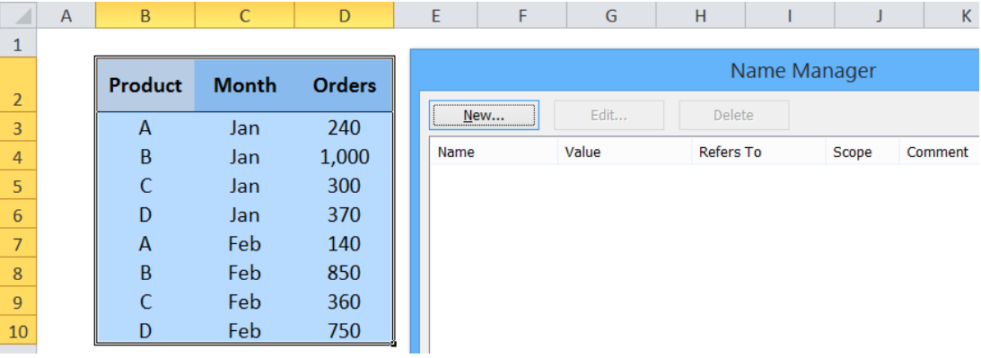Figure 13. Creating a new range

Step 3. Let us name the range “Data”.  In the Refers to bar,enter the formula:

=OFFSET(Sheet1!$B$2,0,0,COUNTA(Sheet1!$B:$B),COUNTA(Sheet1!$2:$2))

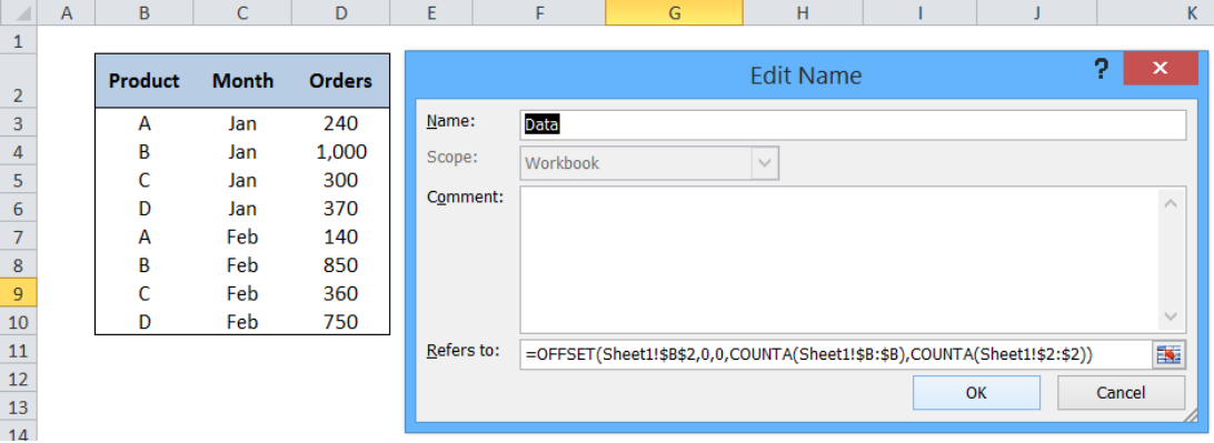Figure 14. Entering the formula for dynamic range

Where

• Our reference cell is B2
• The offset is 0 rows and 0 columns, which means that our reference is still cell B2
• The number of rows is determined by the COUNTA function: COUNTA(Sheet1!$B:$B) which returns the number if non-empty rows in column B
• The number of columns is determined by the COUNTA function: COUNTA(Sheet1!$2:$2) which returns the number if non-empty columns in row 2

Pivot Table Having a Dynamic Range

Now that we have created a dynamic range, let’s see how it improves our pivot table.

Step 1.  Click the Insert tab and select PivotTable.

Step 2. In the Table/Range: bar, enter the name of our dynamic range “Data”.  

Step 3.  Tick Existing Worksheet

Step 4. Click the bar for Location bar, then click cell F3.  

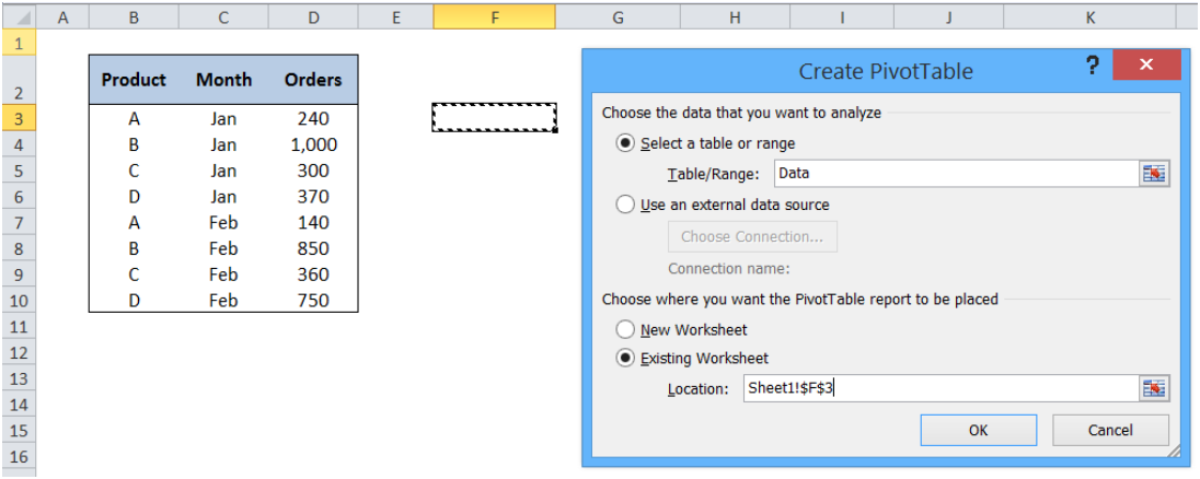Figure 15. Inserting a pivot table with dynamic range

Note:

We do not want to position our pivot table in row 2 to avoid complicating our dynamic range. Note that in our dynamic range formula, we set the number of columns by counting the non-empty cells in row 2.

Step 5.  Create our pivot table by clicking Product and Orders, then dragging Month into the column labels.

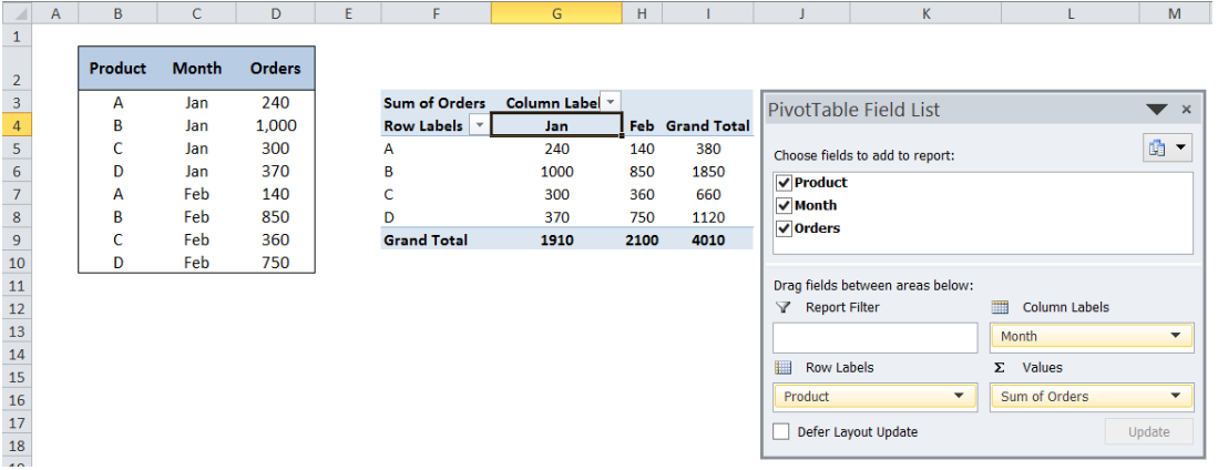Figure 16. Creating our pivot table

Step 6. Now we add more rows into our source table.  Add the March data as shown below. Then press  Ctrl + Alt + F to refresh the  pivot table.

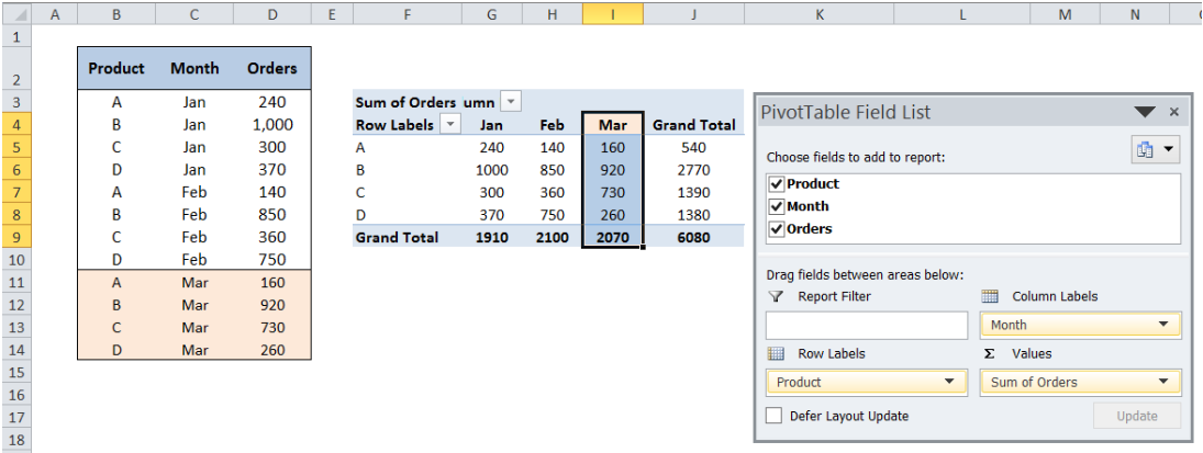Figure 17. Pivot table automatically expands with more data

The pivot table expands with the data.

Step 7. Now let’s try and remove some values in our source table.

Delete the column “Month” then  press Ctrl + Alt + F to refresh.  

The pivot table automatically shrinks with our data, showing only the Sum of Orders.  .

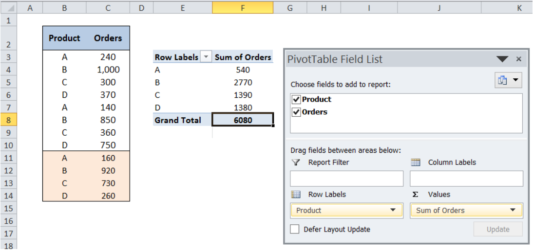Figure 18. Pivot table automatically shrinks with less data

With a dynamic range, working with pivot tables becomes easier and more manageable.  We can shrink and expand our pivot table effortlessly with any changes in our data.

Most of the time, the problem you will need to solve will be more complex than a simple application of a formula or function. If you want to save hours of research and frustration, try our live Excelchat service! Our Excel Experts are available 24/7 to answer any Excel question you may have. We guarantee a connection within 30 seconds and a customized solution within 20 minutes.