

What is a Pivot Table?
A Pivot Table is a table that we can use for analyzing, summarizing, and calculating data that enables us to visualize trends, comparisons, and patterns in our data in a condensed manner. A Pivot Table is useful for organizing a large amount of data in Microsoft Excel.
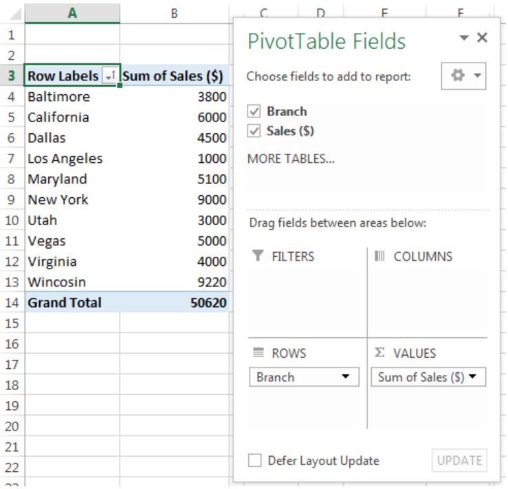 Figure 1- Created Pivot Table
Components of a Pivot Table
A Pivot Table is made of:
- Rows
- Columns
- Data fields
- Pages
We can move these components around and it helps us to isolate, sum, expand, and place data into groups in real time.
Employing the Pivot Table
When we have a particular data (the Data must be labeled with headings) that has been labeled, the Pivot Table converts each header of the data into a data option that can be manipulated by us. We have the liberty to remove or add columns containing data.
Benefits of Using the Pivot Table
- Ease of Use – Pivot tables are easy to understand. We can easily summarize our data by dragging the columns to our chosen section of the table.
- Easy Data Analysis – We can analyze a “super-bulky” data with Pivot Tables in one fell swoop. Pivot Tables enables us to filter data we do not want from a large data.
- Quick and Easy Summary of Data – Pivot Tables helps us to reduce a bulky data that is difficult to understand into a comprehensible piece. We can quickly make an informed summary of our data with Pivot Tables.
- Forecasting – With Pivot Tables, we can see trends or patterns in our data. With this, we can make an accurate forecast.
- External Source Link Integration – Apart from creating reports quickly and saving time, Pivot Tables allows us to make use of links from external sources.
How to Create a Pivot Table in Excel
The steps below will walk through the process of Inserting a Pivot Table in Excel.
Setting up the Data
- We will create a Pivot Table with the Data in figure 2.
 Figure 2 – Setting up the Data
Creating the Pivot Table
- We will select the range (B3:C13) of the table
- We will click on the Insert tab and click on Pivot Table
 Figure 3- Clicking on Pivot Table
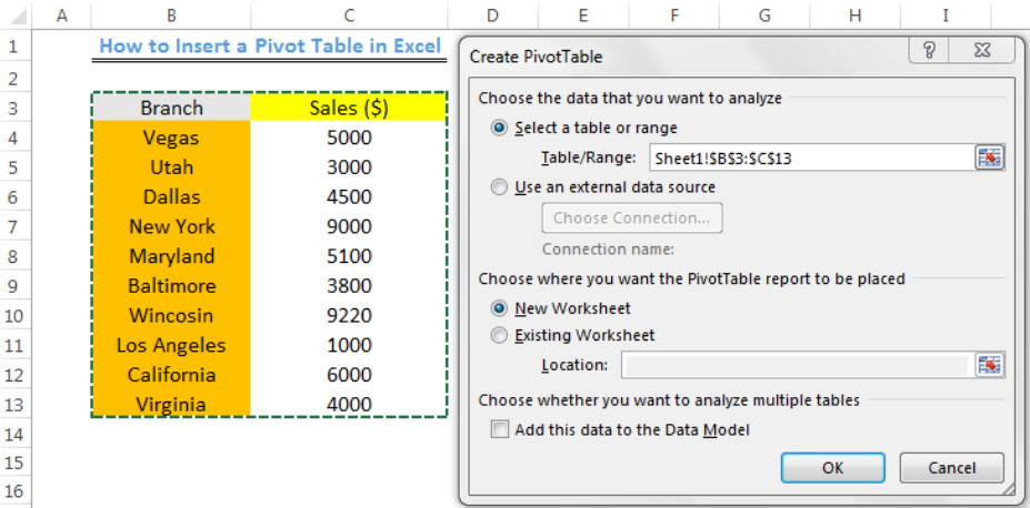 Figure 4- Creating the Pivot Table
- We will click on OK to create the Pivot Table in a New Worksheet
- We will select the fields we want to add to the Pivot Table
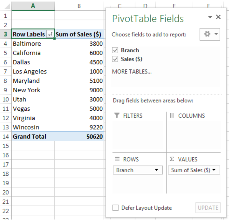 Figure 5- Created Pivot Table
- We can also add a little change to the Pivot Table by dragging the Sales ($) in the Choose fields to add to report to the COLUMNS beside FILTERS
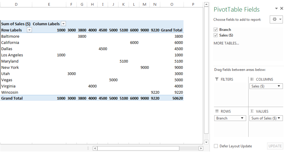 Figure 6- Pivot Table
Alternative
- We can click on anywhere on the table, click on the Insert tab, and click on Table as shown in figure 3.
 Figure 7- Alternative method of Creating a Pivot Table
- We will click on OK
 Figure 8- Alternative method of Creating a Pivot Table
- Once we have this table (this is not the Pivot Table), we can either follow the process of figure 3 to insert the Pivot Table or Click on “Summarize with PivotTable” below Insert as shown in figure 8. We will arrive at figure 4 and can proceed as already discussed.
Note
- Under “Choose where you want the PivotTable report to be placed”, we can specify the location where we want the worksheet to be placed. Assuming we select “Existing Worksheet”, a valid location will be an unoccupied cell in the existing worksheet, e.g. Sheet1!$D$3
- No cell within the range of the table should be completely left blank
Instant Connection to an Expert through our Excelchat Service
Most of the time, the problem you will need to solve will be more complex than a simple application of a formula or function. If you want to save hours of research and frustration, try our live Excelchat service! Our Excel Experts are available 24/7 to answer any Excel question you may have. We guarantee a connection within 30 seconds and a customized solution within 20 minutes.


Leave a Comment