Excel formula: Hyperlink to first match

Hyperlink to first match

Excel offers many tips and tricks to help its users. One of them is to create a hyperlink to the first match. We can use the HYPERLINK, CELL, INDEX and MATCH functions to create a hyperlink to the first match. It extracts the first match in a lookup and creates the hyperlink for that match. In this article, we will learn how to create a hyperlink to the first match in Excel.

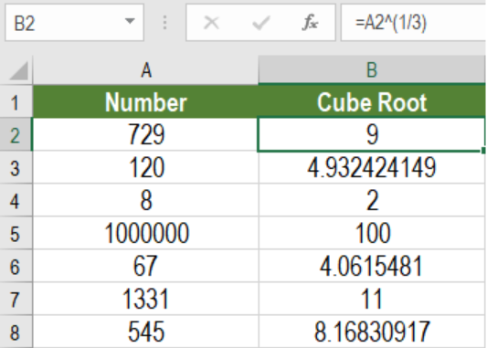Figure 1. Example of How to Hyperlink to the First Match

Generic Formula

=HYPERLINK("#"&CELL("address",INDEX(range,MATCH(val,range,0))),val)

This formula is uses the HYPERLINK function as its core. The other functions used are CELL, INDEX and MATCH. It creates a hyperlink to the first match on the lookup value in the range.

How this formula works

Here, we use an INDEX and MATCH function to extract the first match of the lookup value in the range. The position of the value found inside the range is extracted by the MATCH function. Excel passes this position value to the INDEX function as row_num argument. The range is provided as the array argument. The INDEX function returns the address of this value. We find this address using the CELL function and concatenate it to the “#” character. Then, we provide this concatenated value to the HYPERLINK function as the link_location. The HYPERLINK function builds a clickable link to the cell address within the same sheet.

Setting Up Data

The following example uses a fruit sales data set. Column A has the name of the fruits. Column B has the sales.

Figure 2. The Fruit Sales Data Set

To create hyperlinks to the first match of the fruits in column E, we need to:

Go to Cell E9 and click on it with our mouse.
Assign the formula =HYPERLINK("#"&CELL("address",INDEX($A$2:$A$20,MATCH(D9,$A$2:$A$20,0))),D9) in cell E3.
Next, we need to press Enter to assign the formula to cell E9.

Figure 3. Applying the formula to the Data

Lastly, we need to drag the formula from cells E9 to E12 to copy the formula to the entire column.

This will create clickable links on column E that will redirect to the first match of the fruit names in column A.

Most of the time, the problem you will need to solve will be more complex than a simple application of a formula or function. If you want to save hours of research and frustration, try our live Excelchat service! Our Excel Experts are available 24/7 to answer any Excel question you may have. We guarantee a connection within 30 seconds and a customized solution within 20 minutes.

Did this post not answer your question? Get a solution from connecting with the expert.

Another blog reader asked this question today on Excelchat:

I'm using an index/match formula. My problem is that there are multiple matches, so the formula is returning the first one it finds. I need the formula to return the first one it finds, then on the next line, return the subsequent match (ignoring the first match).

An Excelchat Expert solved this problem in 12 mins!

Hi there, I'm looking for a formula to match a text within an array and return the results found. I know how to you use vlookup/match/index formula's, but I can only return the first match found. I would like to return the first match in cell A1 and the second match inside A2, third inside A3, etc. So when the first match is found and placed inside A1 then the formula inside A2 should ignore the first match that is already found and show the next match value. I would like to get this done with a formula and not with the autofilter option inside Excel.

An Excelchat Expert solved this problem in 29 mins!

Need to generate a new column using a SQl which generates a hyperlink and exports it with a hyperlink alias (Keeping the hyperlink active) to excel. This exports the following output for link column: =HYPERLINK("http://mycompany.com/order/1","[Notes]") Excel does not automatically consider the output as a formula.

An Excelchat Expert solved this problem in 25 mins!