

While working with Excel, we are able to display pre-sorted values in a certain order by using the INDEX, MATCH and ROWS functions. This step by step tutorial will assist all levels of Excel users in displaying sorted values with the aid of a helper column.
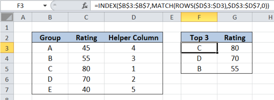 Figure 1. Final result: Display sorted values with helper column
Formula for Top Group : =INDEX($B$3:$B$7,MATCH(ROWS($D$3:$D3),$D$3:$D$7,0))
Formula for Top Rating : =INDEX($C$3:$C$7,MATCH(ROWS($D$3:$D3),$D$3:$D$7,0))
Syntax of the INDEX function
INDEX function returns a value from within a range, as specified by the row and column number
=INDEX(array, row_num, column_num)
The parameters are:
- array – a range of cells where we want to retrieve some data
- row_num – the row in the array from which we want to retrieve data
- column_num – the column in the array from which we want to retrieve data; if the array has only one column, column_num can be omitted
Syntax of the MATCH function
MATCH function returns the position of a value in a range
=MATCH(lookup_value, lookup_array, [match_type])
The parameters are:
- lookup_value – a value which we want to find in the lookup_array
- lookup_array – the range of cells containing the value we want to match
- [match_type] – optional; the type of match; if omitted, the default value is 1; We use 0 to find an exact match
Syntax of the ROWS function
ROWS function returns the number of rows in a data set
=ROW(array)
- array– an array, range or reference for which we want to determine the number of rows
Setting up Our Data
Our table contains three columns: Group (column B), Rating (column C) and a Helper Column (column D). A helper column is a column we set-up to help simplify a set of data. In column D, we determine the rank of the groups by rating from 1 to 5, with 1 being the highest.
In column F, we want to find the top 3 groups in the order of 1, 2 and 3. In column G, we want to find the corresponding rating for each of the top 3 groups.
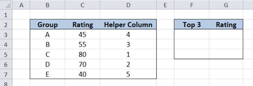 Figure 2. Sample data to display sorted values with helper column
Display top 3 groups
We want to identify the top 3 groups and display them in proper order in column F, with the help of our helper column (column D). Let us follow these steps:
Step 1. Select cell F3
Step 2. Enter the formula: =INDEX($B$3:$B$7,MATCH(ROWS($D$3:$D3),$D$3:$D$7,0))
Step 3: Press ENTER
Step 4: Copy the formula in cell F3 to cells F4:F5 by clicking the “+” icon at the bottom-right corner of cell F3 and dragging it down
The dollar signs “$” in the formula fix the cells so that we can easily copy and paste the formula to other cells.
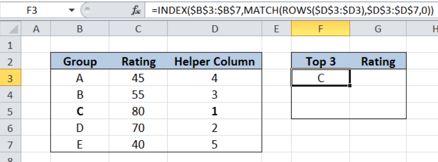 Figure 3. Entering the formula using INDEX, MATCH and ROWS
Our array for the INDEX function is the range B3:B7. Since there is only one column, we can omit the column_num in our formula. The row_num is determined by the MATCH function : MATCH(ROWS($D$3:$D3),$D$3:$D$7,0)
Our lookup_value for the MATCH function is ROWS($D$3:$D3), which returns the number of rows of D3:D3, whose value is 1. Hence, we want to match the value 1 in the lookup_array D3:D7 {4;3;1;2;5}. The value 1 is the third value in the array so the MATCH function returns 3.
Finally, the INDEX function returns the third row in the range B3:B7, which is B5, or “C”. The result displayed in cell F3 is group C, which is also the top 1 group with the highest rating.
Copying the formula to cells F4 and F5 will return the top 2 and top 3 groups. Below table displays the top 3 groups sorted according to rating.
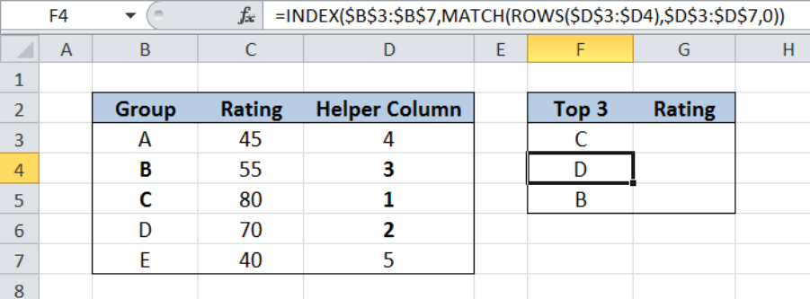 Figure 4. Output: Display top 3 groups sorted from highest rating
Display top 3 ratings
Now that we’ve identified the top 3 groups, we want to find the corresponding ratings. The formula is quite similar to our previous example. We only have to change the array for our INDEX function to the range C3:C7, instead of B3:B7.
Let us follow these steps:
Step 1. Select cell G3
Step 2. Enter the formula: =INDEX($C$3:$C$7,MATCH(ROWS($D$3:$D3),$D$3:$D$7,0))
Step 3: Press ENTER
Step 4: Copy the formula in cell G3 to cells G4:G5 by clicking the “+” icon at the bottom-right corner of cell G3 and dragging it down
Our formula returns the value in column C based on the row number given by the MATCH and ROWS functions.
Below table displays the ratings of the top 3 groups.
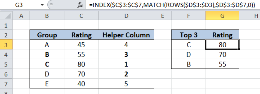 Figure 5. Output: Display top 3 ratings sorted from highest value
Most of the time, the problem you will need to solve will be more complex than a simple application of a formula or function. If you want to save hours of research and frustration, try our live Excelchat service! Our Excel Experts are available 24/7 to answer any Excel question you may have. We guarantee a connection within 30 seconds and a customized solution within 20 minutes.


Leave a Comment